---
header-includes:
- \usepackage{float}
---
```{r}
library(dplyr)
library(purrr)
library(knitr)
library(magrittr)
library(stringr)
library(ggplot2)
knitr::opts_chunk$set(out.width = "85%")
```
# Figures {#sec-appendix-figures}
## IRR Analyses
```{r}
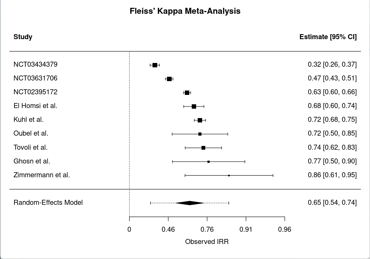
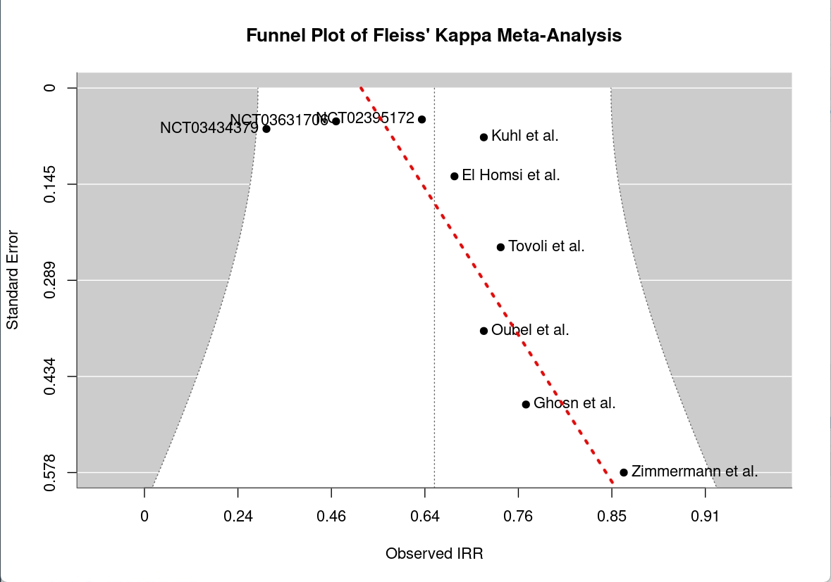
#| label: fig-irr-meta-analysis-fleiss-results
#| fig-cap: "Fleiss' kappa results and funnel plot for the inter-rater reliability (IRR) meta-analysis."
#| fig-subcap: ["Fleiss' kappa results", "Fleiss' kappa funnel plot"]
#| fig-pos: 'H'
#| out-width: "85%"
knitr::include_graphics(c(
"images/irr_meta_analysis/fleiss_results.png",
"images/irr_meta_analysis/fleiss_funnel.png"
))
```
```{r}
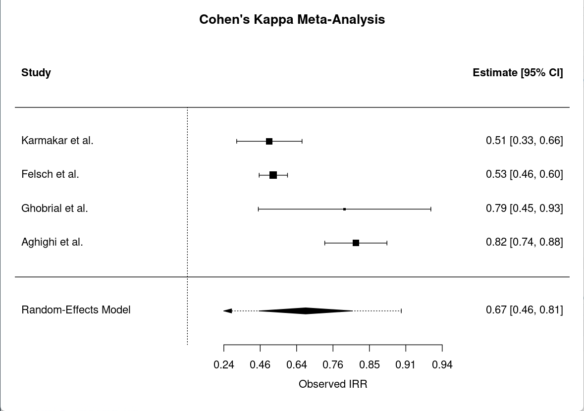
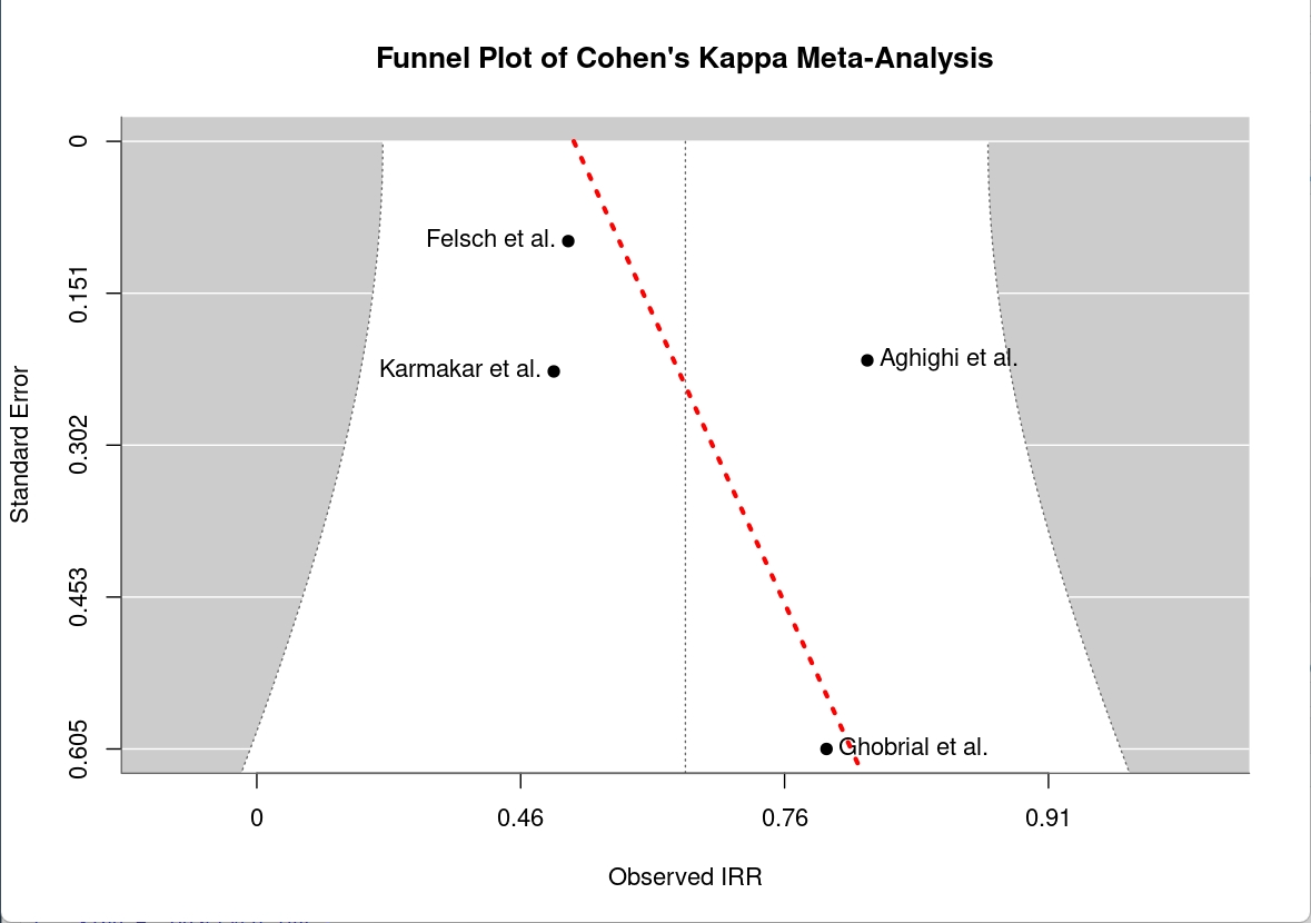
#| label: fig-irr-meta-analysis-cohen-results
#| fig-cap: "Cohen's kappa results and funnel plot for the inter-rater reliability (IRR) meta-analysis."
#| fig-subcap: ["Cohen's kappa results", "Cohen's kappa funnel plot"]
#| fig-pos: 'H'
#| out-width: "85%"
knitr::include_graphics(c(
"images/irr_meta_analysis/cohen_results.png",
"images/irr_meta_analysis/cohen_funnel.png"
))
```
## Trial Results
### Overall Agreement
#### Estimated Marginal Means (EMMs)
::: {.landscape}
```{r}
#| label: tbl-orr-overall-emmeans
#| tbl-cap: "Estimated marginal means (EMMs) between all raters for the objective response rate (ORR) analyses"
readRDS("data/lme_overall_results.rds") %>%
extract2("lme_contrasts_table_only") %>%
bind_rows(.id = "Study") %>%
mutate(
across(estimate:t.ratio, ~round(.x, 4) ),
p.value = round(p.value, 4)
) %>%
mutate(
p.value = paste0(p.value, "$^{", gtools::stars.pval(p.value), "}$")
) %>%
mutate(
contrast = str_replace_all(contrast, "SITE INVESTIGATOR", "Site Inv."),
contrast = tools::toTitleCase(tolower(contrast))
) %>%
rename(Contrast = contrast, Estimate = estimate) %>%
kable()
```
:::
#### LME Equations
```{r}
#| echo: false
#| results: 'asis'
cat("$$", readRDS('data/lme_overall_results.rds') %>% extract2('lme_latex_equations') %>% extract2(1), "$$ {#eq-orr-emmeans-study1}")
```
Equation: Estimated marginal means for the objective response rate (ORR) for study NCT02395172.
```{r}
#| echo: false
#| results: 'asis'
cat("$$\n", readRDS('data/lme_overall_results.rds') %>% extract2('lme_latex_equations') %>% extract2(2), "\n$$ {#eq-orr-emmeans-study2}")
```
Equation: Estimated marginal means for the objective response rate (ORR) for study NCT03434379.
```{r}
#| echo: false
#| results: 'asis'
cat("$$\n", readRDS('data/lme_overall_results.rds') %>% extract2('lme_latex_equations') %>% extract2(3), "\n$$ {#eq-orr-emmeans-study3}")
```
Equation: Estimated marginal means for the objective response rate (ORR) for study NCT03631706.
### Objective Response Rate Results
#### McNemar's Tests
```{r}
orr_data <- readRDS("data/orr_cochrans_mcnemars.rds")
```
```{r}
#| label: tbl-orr-cochrans-q-contingency-tables-NCT02395172
#| tbl-cap: "Contingency tables for the McNemar's tests study NCT02395172."
#| tbl-pos: 'H'
orr_data$orr_mcnemars_tests$NCT02395172$two_way_tables
```
```{r}
#| label: tbl-orr-cochrans-q-contingency-tables-NCT03434379
#| tbl-cap: "Contingency tables for the McNemar's tests study NCT03434379."
#| tbl-pos: 'H'
orr_data$orr_mcnemars_tests$NCT03434379$two_way_tables
```
```{r}
#| label: tbl-orr-cochrans-q-contingency-tables-NCT03631706
#| tbl-cap: "Contingency tables for the McNemar's tests study NCT03631706."
#| tbl-pos: 'H'
orr_data$orr_mcnemars_tests$NCT03631706$two_way_tables
```
\newpage
### Survival Analyses {#sec-appendix-survival-analyses}
\newpage
#### Time to Progression (TTP) Analyses {#sec-appendix-ttp-analyses}
##### NCT02395172
```{r}
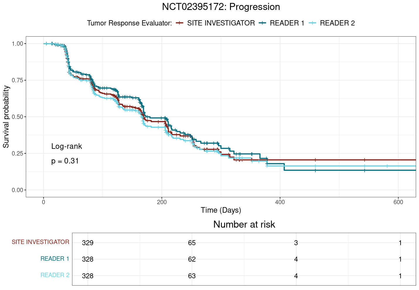
#| label: fig-ttp-nct02395172-km
#| fig-cap: "Kaplan-Meier survival plot for time to progression (TTP) for study NCT02395172."
#| fig-pos: 'H'
knitr::include_graphics(
"./images/survival_images/NCT02395172_progression_kaplan_meier.png"
)
```
```{r}
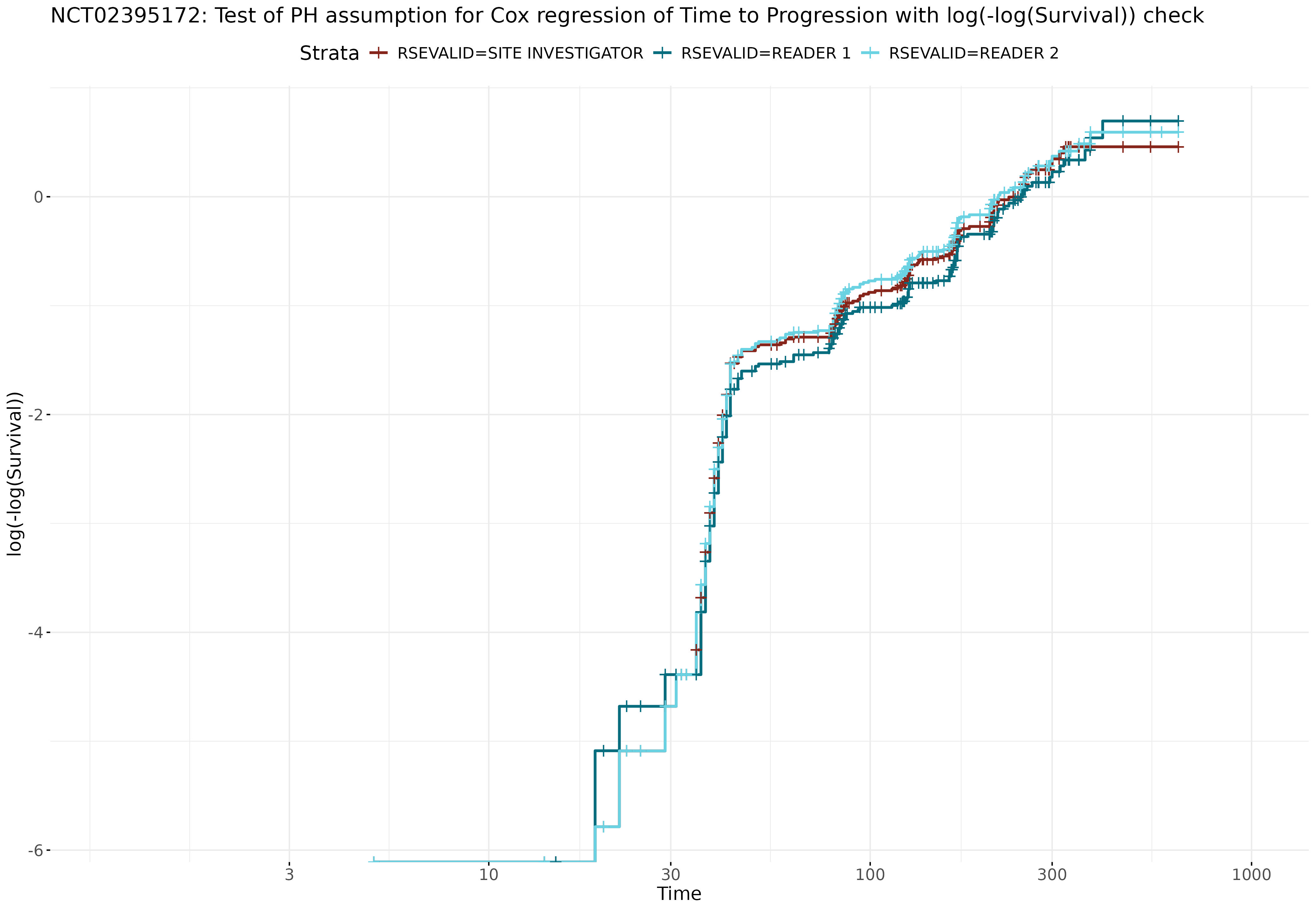
#| label: fig-ttp-nct02395172-cloglog
#| fig-cap: "Log-minus-log survival plot for time to progression (TTP) for study NCT02395172."
#| fig-pos: 'H'
knitr::include_graphics(
"./images/survival_images/NCT02395172_progression_cox_cloglog.jpeg"
)
```
```{r}
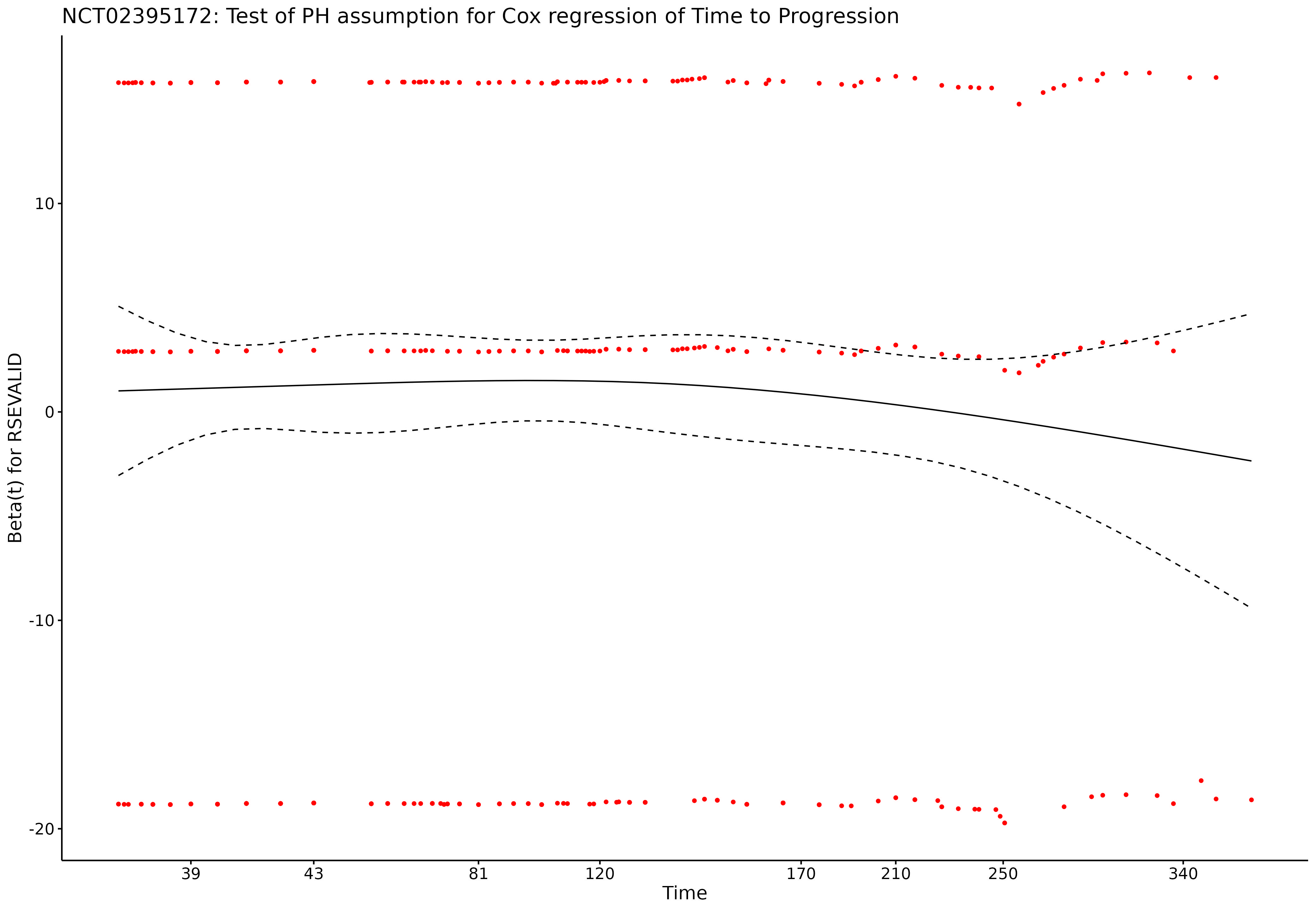
#| label: fig-ttp-nct02395172-cox-zph
#| fig-cap: "Schoenfeld residuals for the Cox proportional hazards model for time to progression (TTP) for study NCT02395172."
#| fig-pos: 'H'
knitr::include_graphics(
"./images/survival_images/NCT02395172_progression_cox_zph.jpeg"
)
```
##### NCT03434379
```{r}
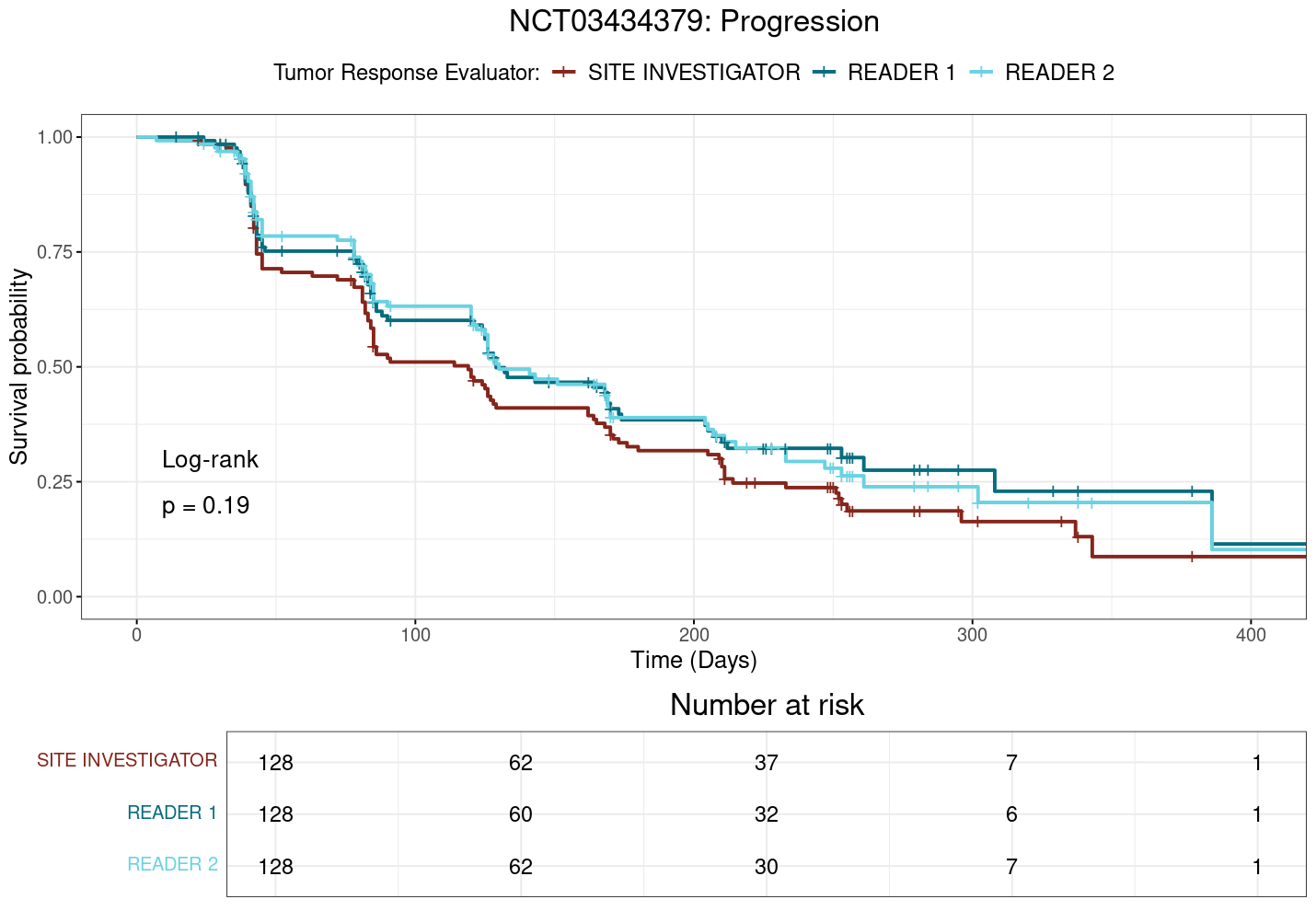
#| label: fig-ttp-nct03434379-km
#| fig-cap: "Kaplan-Meier survival plot for time to progression (TTP) for study NCT03434379."
#| fig-pos: 'H'
knitr::include_graphics(
"./images/survival_images/NCT03434379_progression_kaplan_meier.png"
)
```
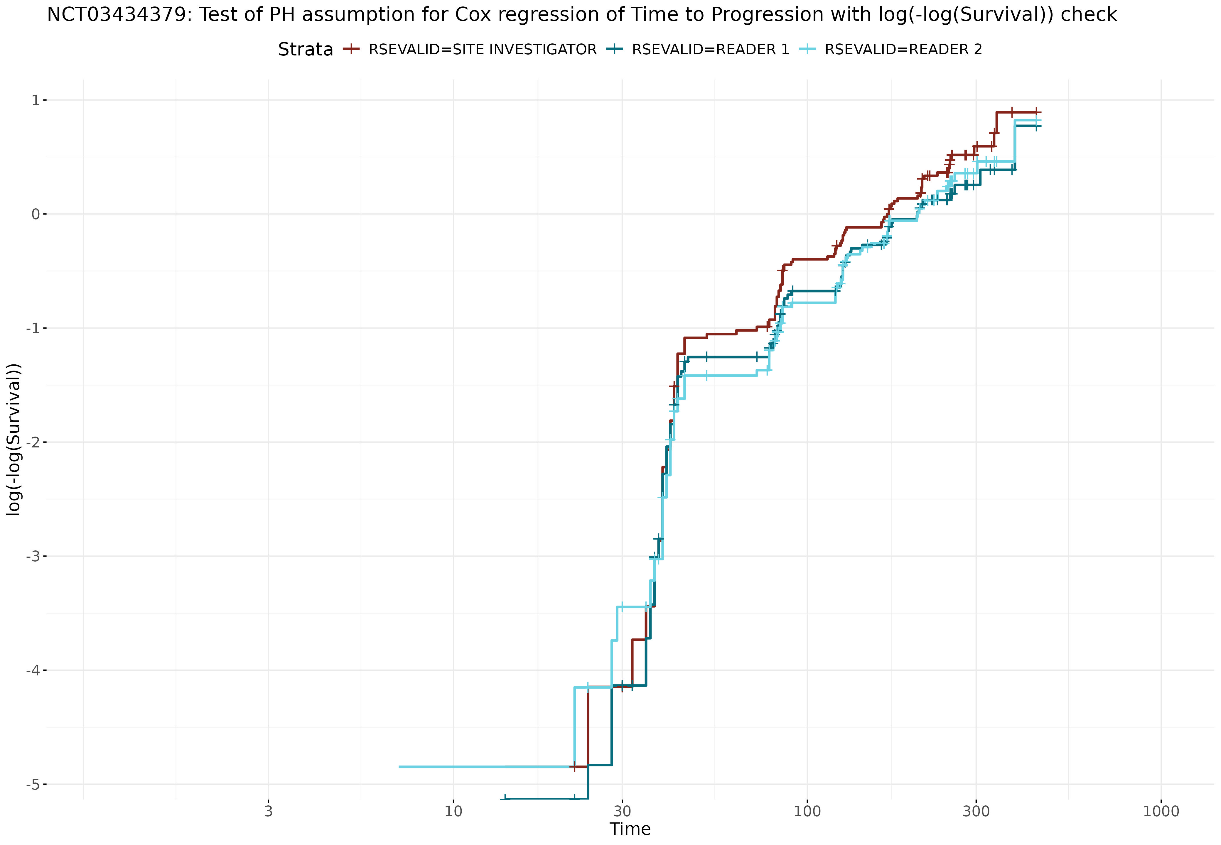
```{r}
#| label: fig-ttp-nct03434379-cloglog
#| fig-cap: "Log-minus-log survival plot for time to progression (TTP) for study NCT03434379."
#| fig-pos: 'H'
knitr::include_graphics(
"./images/survival_images/NCT03434379_progression_cox_cloglog.jpeg"
)
```
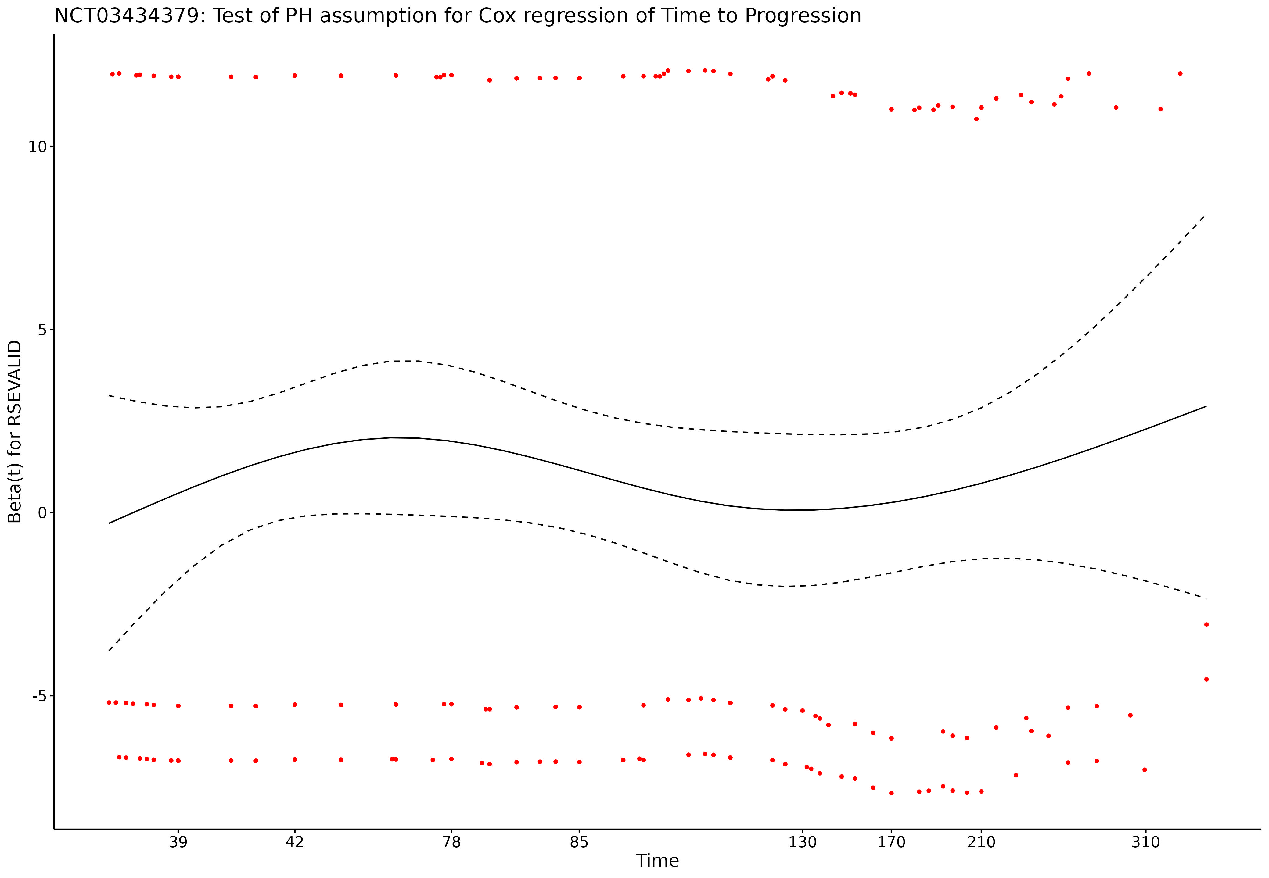
```{r}
#| label: fig-ttp-nct03434379-cox-zph
#| fig-cap: "Schoenfeld residuals for the Cox proportional hazards model for time to progression (TTP) for study NCT03434379."
#| fig-pos: 'H'
knitr::include_graphics(
"./images/survival_images/NCT03434379_progression_cox_zph.jpeg"
)
```
##### NCT03631706
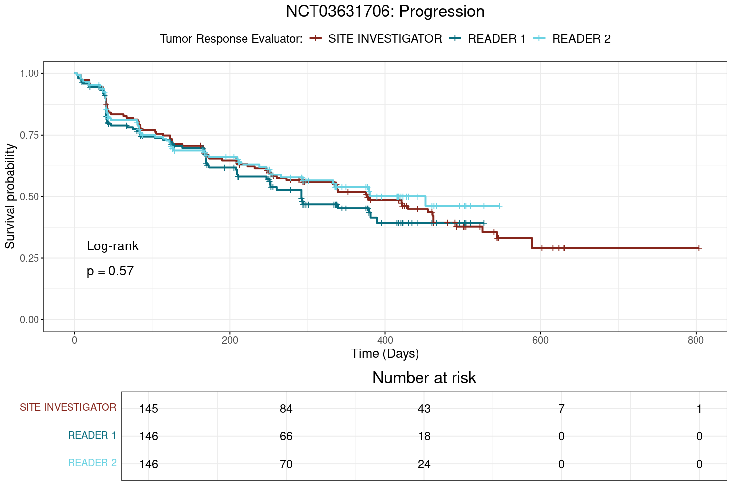
```{r}
#| label: fig-ttp-nct03631706-km
#| fig-cap: "Kaplan-Meier survival plot for time to progression (TTP) for study NCT03631706."
#| fig-pos: 'H'
knitr::include_graphics(
"./images/survival_images/NCT03631706_progression_kaplan_meier.png"
)
```
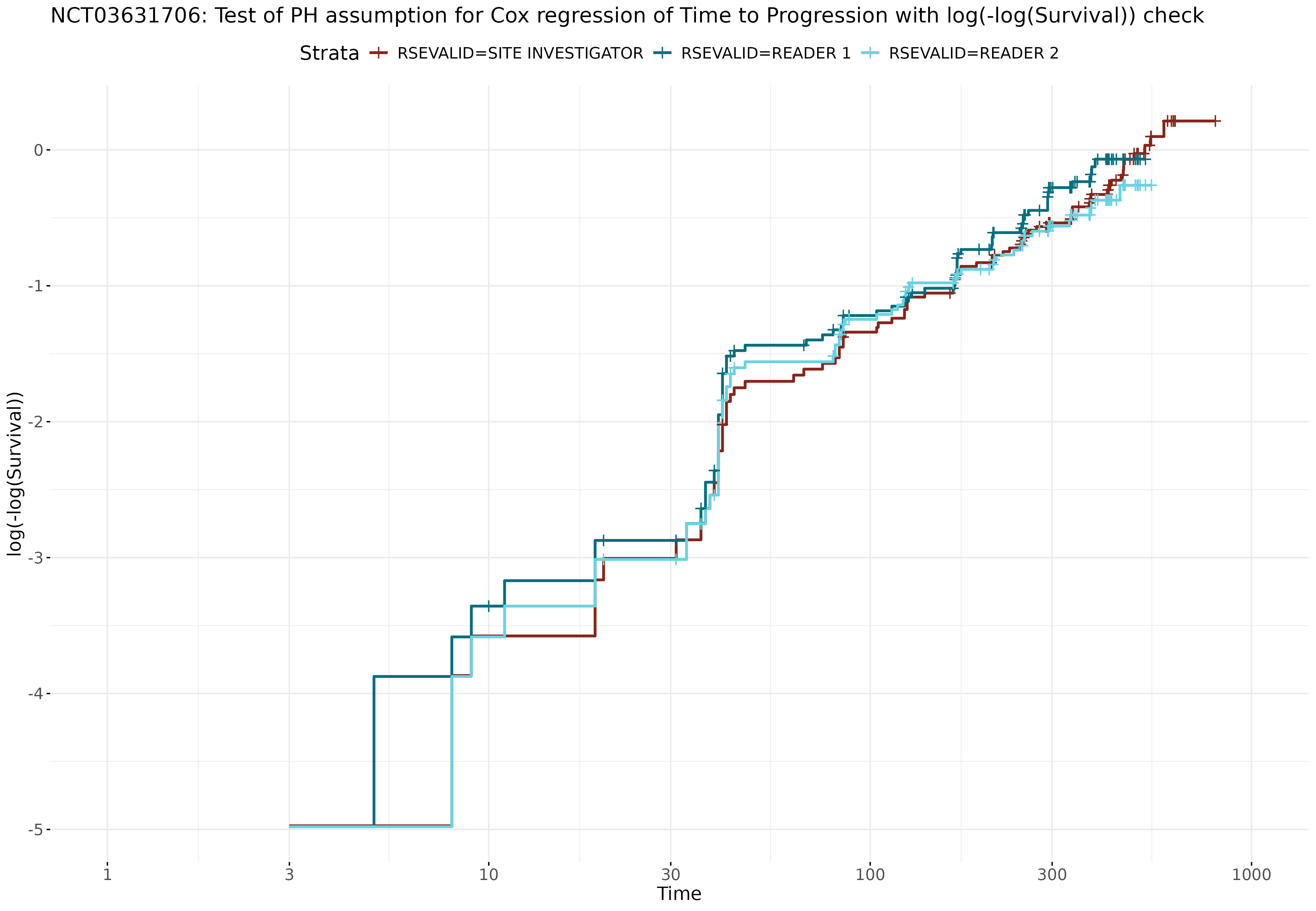
```{r}
#| label: fig-ttp-nct03631706-cloglog
#| fig-cap: "Log-minus-log survival plot for time to progression (TTP) for study NCT03631706."
#| fig-pos: 'H'
knitr::include_graphics(
"./images/survival_images/NCT03631706_progression_cox_cloglog.jpeg"
)
```
```{r}
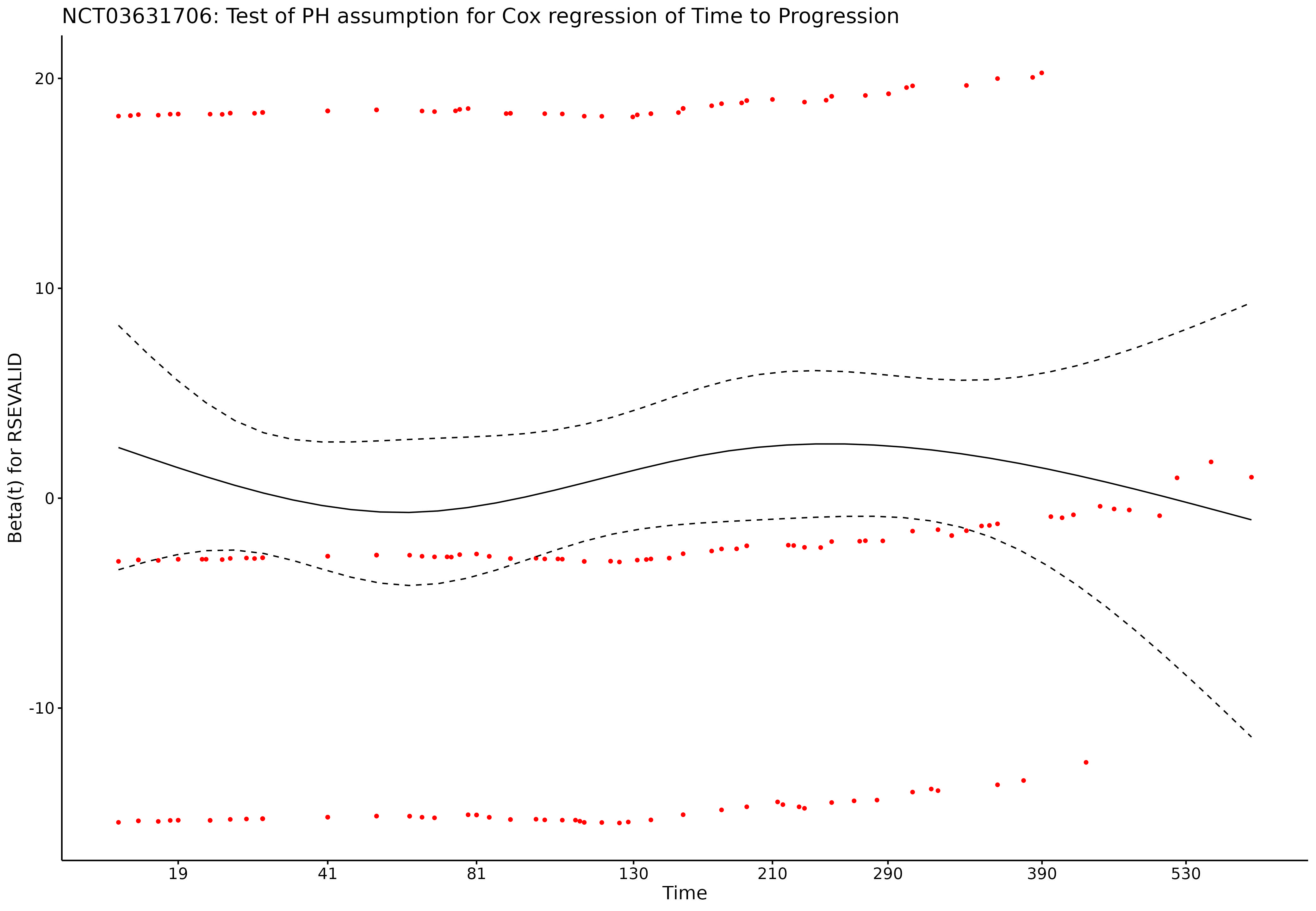
#| label: fig-ttp-nct03631706-cox-zph
#| fig-cap: "Schoenfeld residuals for the Cox proportional hazards model for time to progression (TTP) for study NCT03631706."
#| fig-pos: 'H'
knitr::include_graphics(
"./images/survival_images/NCT03631706_progression_cox_zph.jpeg"
)
```
\newpage
#### Time to Response (TTR) Analyses {#sec-appendix-ttr-analyses}
##### NCT02395172
```{r}
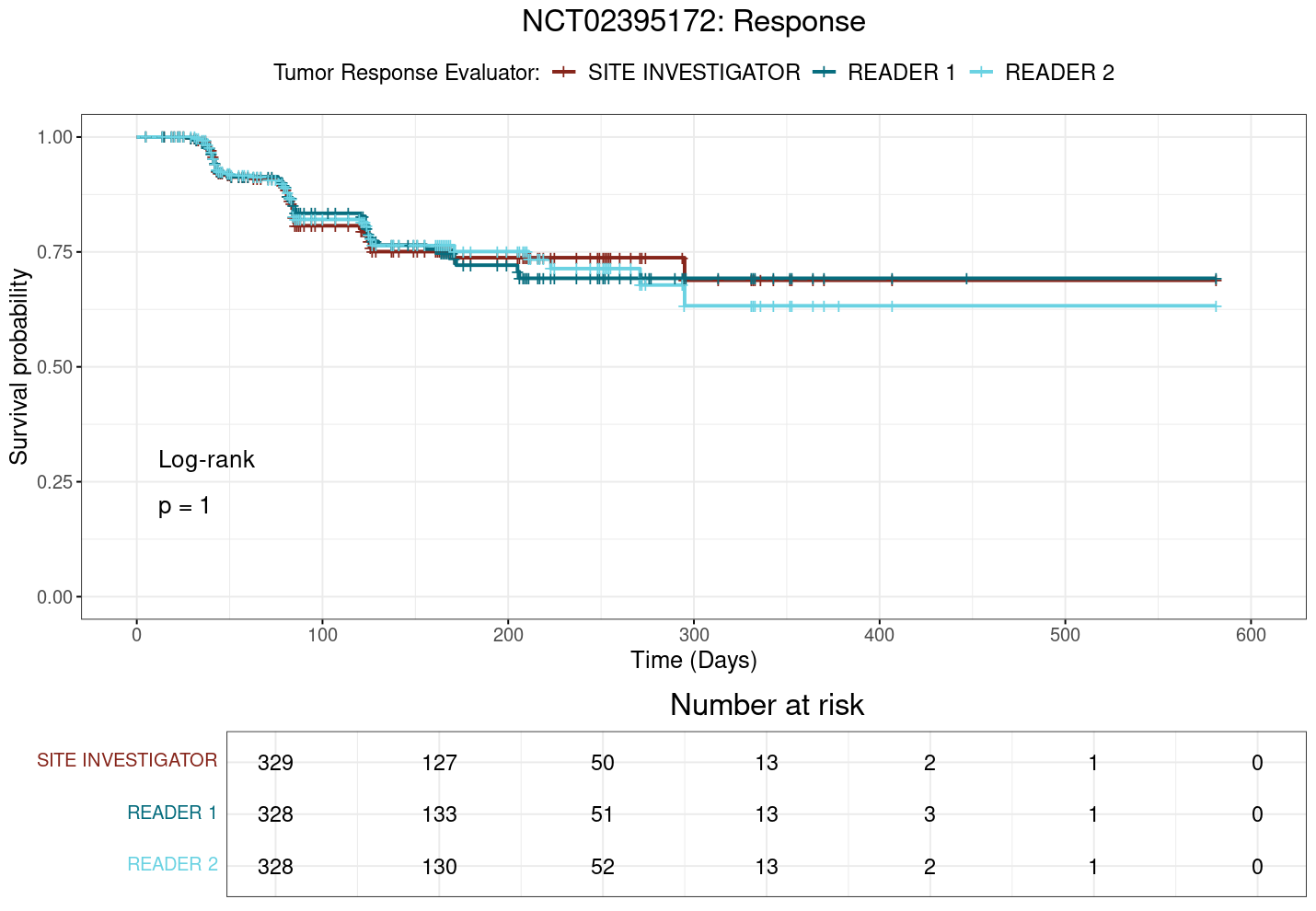
#| label: fig-ttr-nct02395172-km
#| fig-cap: "Kaplan-Meier survival plot for time to response (TTR) for study NCT02395172."
#| fig-pos: 'H'
knitr::include_graphics(
"./images/survival_images/NCT02395172_response_kaplan_meier.png"
)
```
```{r}
#| label: fig-ttr-nct02395172-cloglog
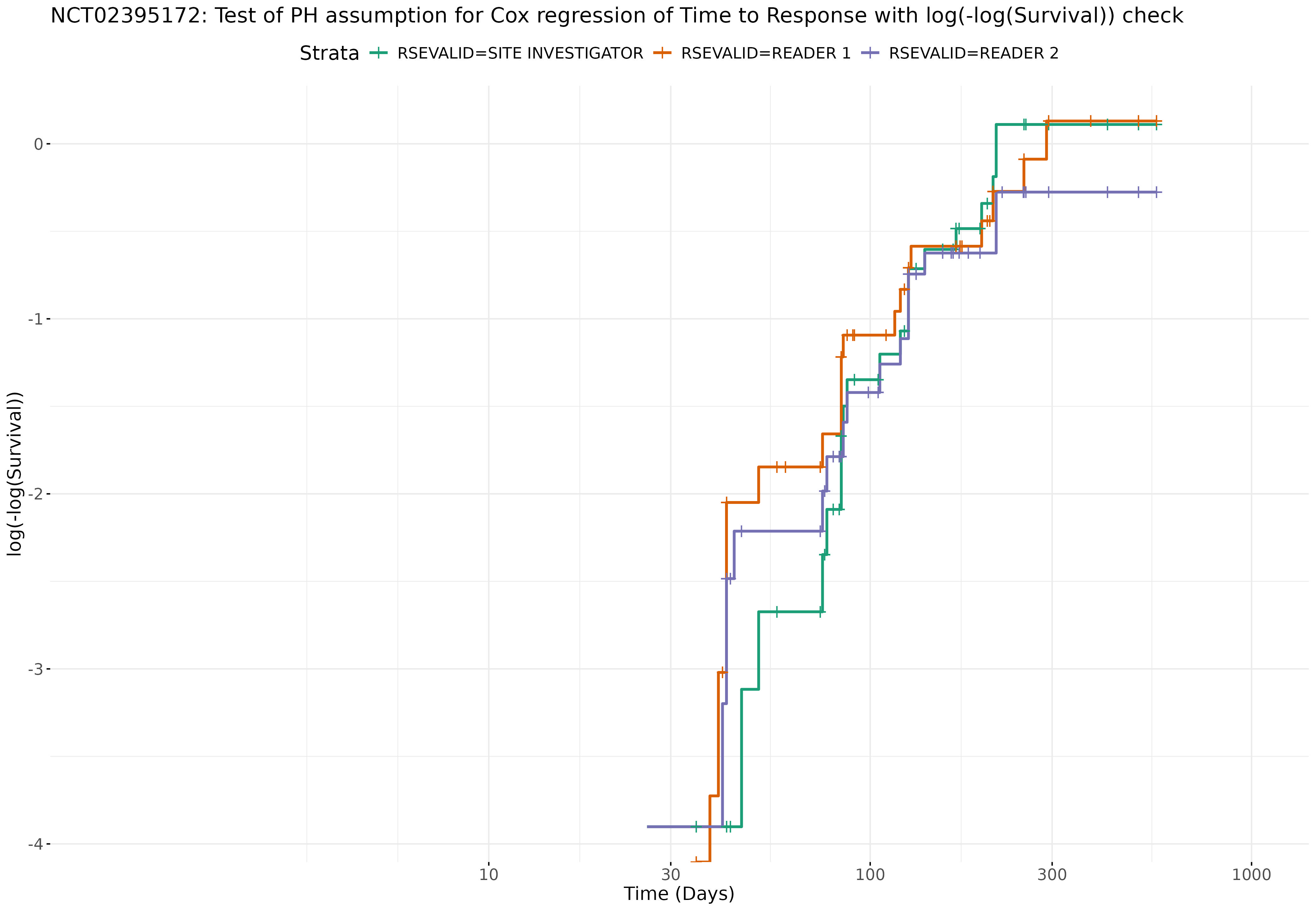
#| fig-cap: "Log-minus-log survival plot for time to response (TTR) for study NCT02395172."
#| fig-pos: 'H'
knitr::include_graphics(
"./images/survival_images/NCT02395172_response_cox_cloglog.jpeg"
)
```
```{r}
#| label: fig-ttr-nct02395172-cox-zph
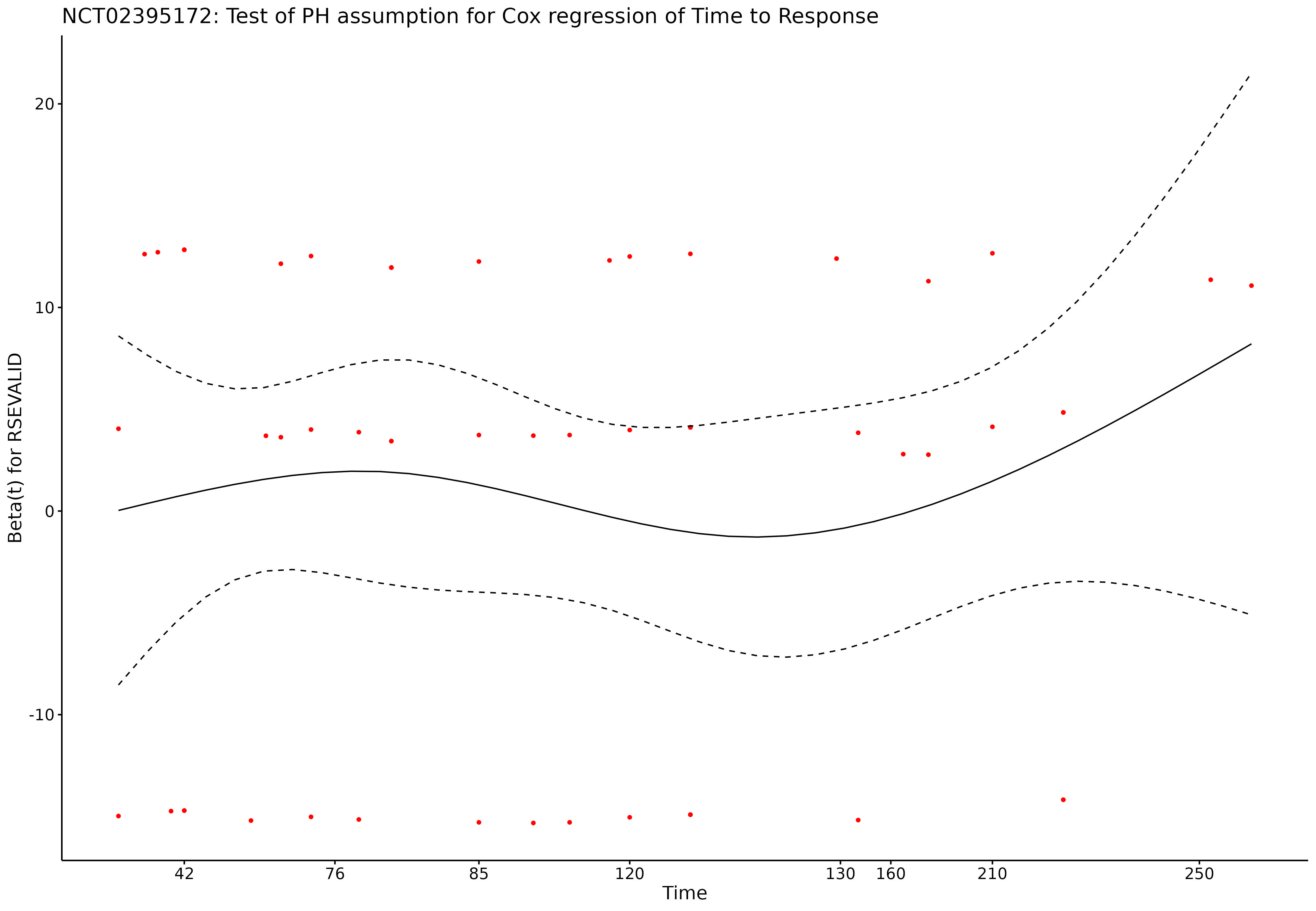
#| fig-cap: "Schoenfeld residuals for the Cox proportional hazards model for time to response (TTR) for study NCT02395172."
#| fig-pos: 'H'
knitr::include_graphics(
"./images/survival_images/NCT02395172_response_cox_zph.jpeg"
)
```
##### NCT03434379
```{r}
#| label: fig-ttr-nct03434379-km
#| fig-cap: "Kaplan-Meier survival plot for time to response (TTR) for study NCT03434379."
#| fig-pos: 'H'
knitr::include_graphics(
"./images/survival_images/NCT03434379_response_kaplan_meier.png"
)
```
```{r}
#| label: fig-ttr-nct03434379-cloglog
#| fig-cap: "Log-minus-log survival plot for time to response (TTR) for study NCT03434379."
#| fig-pos: 'H'
knitr::include_graphics(
"./images/survival_images/NCT03434379_response_cox_cloglog.jpeg"
)
```
```{r}
#| label: fig-ttr-nct03434379-cox-zph
#| fig-cap: "Schoenfeld residuals for the Cox proportional hazards model for time to response (TTR) for study NCT03434379."
#| fig-pos: 'H'
knitr::include_graphics(
"./images/survival_images/NCT03434379_response_cox_zph.jpeg"
)
```
##### NCT03631706
```{r}
#| label: fig-ttr-nct03631706-km
#| fig-cap: "Kaplan-Meier survival plot for time to response (TTR) for study NCT03631706."
#| fig-pos: 'H'
knitr::include_graphics(
"./images/survival_images/NCT03631706_response_kaplan_meier.png"
)
```
```{r}
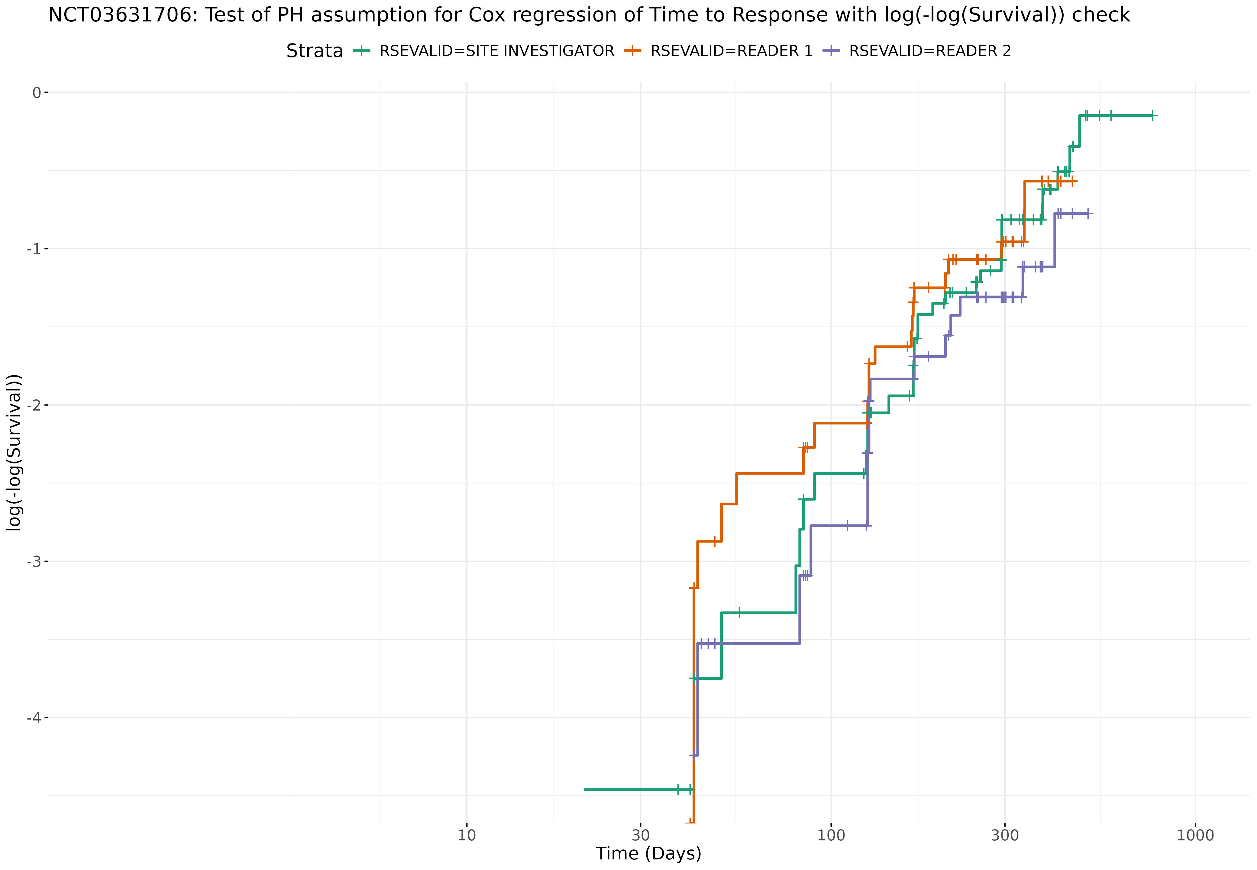
#| label: fig-ttr-nct03631706-cloglog
#| fig-cap: "Log-minus-log survival plot for time to response (TTR) for study NCT03631706."
#| fig-pos: 'H'
knitr::include_graphics(
"./images/survival_images/NCT03631706_response_cox_cloglog.jpeg"
)
```
```{r}
#| label: fig-ttr-nct03631706-cox-zph
#| fig-cap: "Schoenfeld residuals for the Cox proportional hazards model for time to response (TTR) for study NCT03631706."
#| fig-pos: 'H'
knitr::include_graphics(
"./images/survival_images/NCT03631706_response_cox_zph.jpeg"
)
```
\newpage
#### Duration of Response (DoR) Analyses {#sec-appendix-dor-analyses}
##### NCT02395172
```{r}
#| label: fig-dor-nct02395172-km
#| fig-cap: "Kaplan-Meier survival plot for duration of response (DoR) for study NCT02395172."
#| fig-pos: 'H'
knitr::include_graphics(
"./images/survival_images/NCT02395172_dor_kaplan_meier.png"
)
```
```{r}
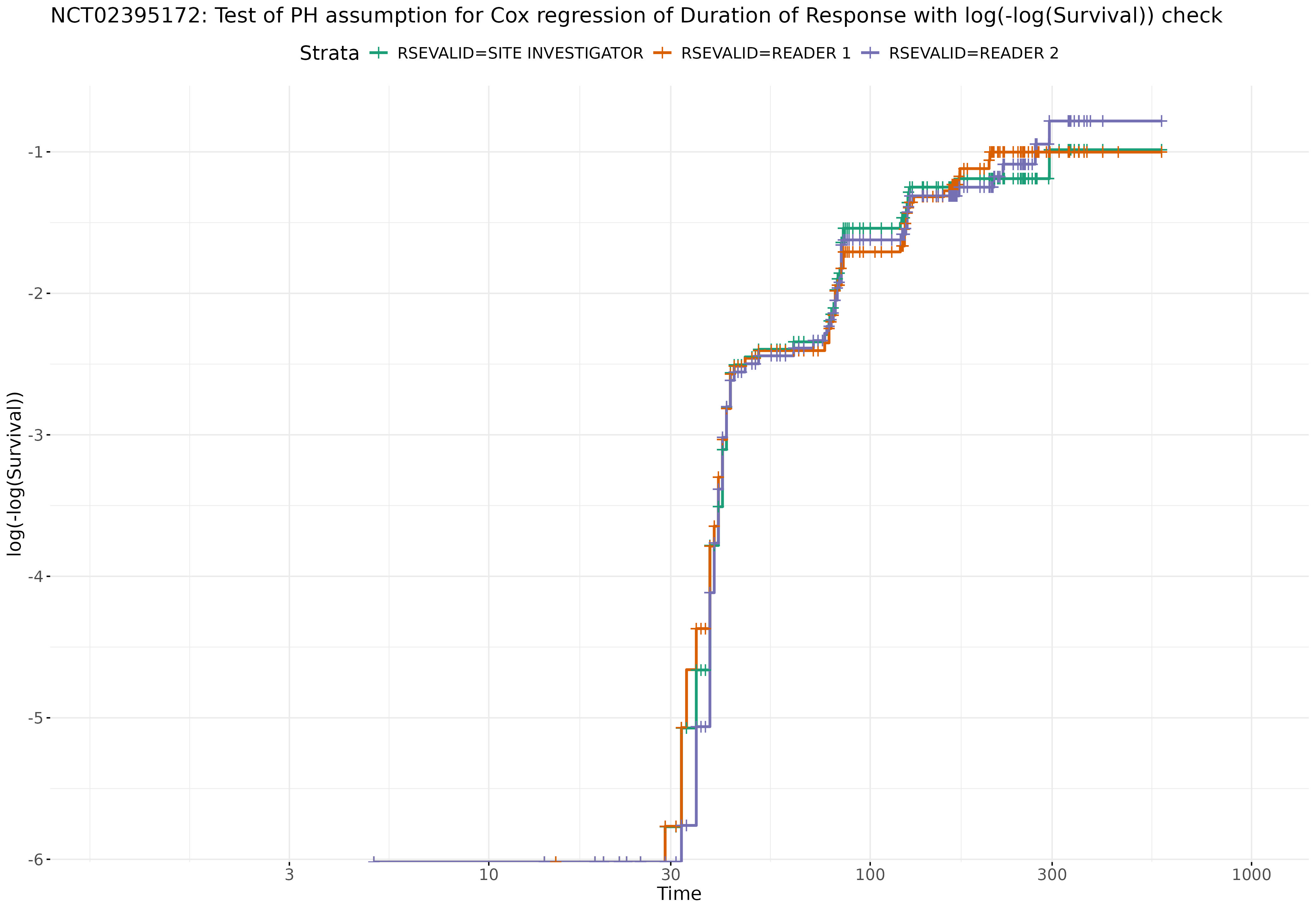
#| label: fig-dor-nct02395172-cloglog
#| fig-cap: "Log-minus-log survival plot for duration of response (DoR) for study NCT02395172."
#| fig-pos: 'H'
knitr::include_graphics(
"./images/survival_images/NCT02395172_dor_cox_cloglog.jpeg"
)
```
```{r}
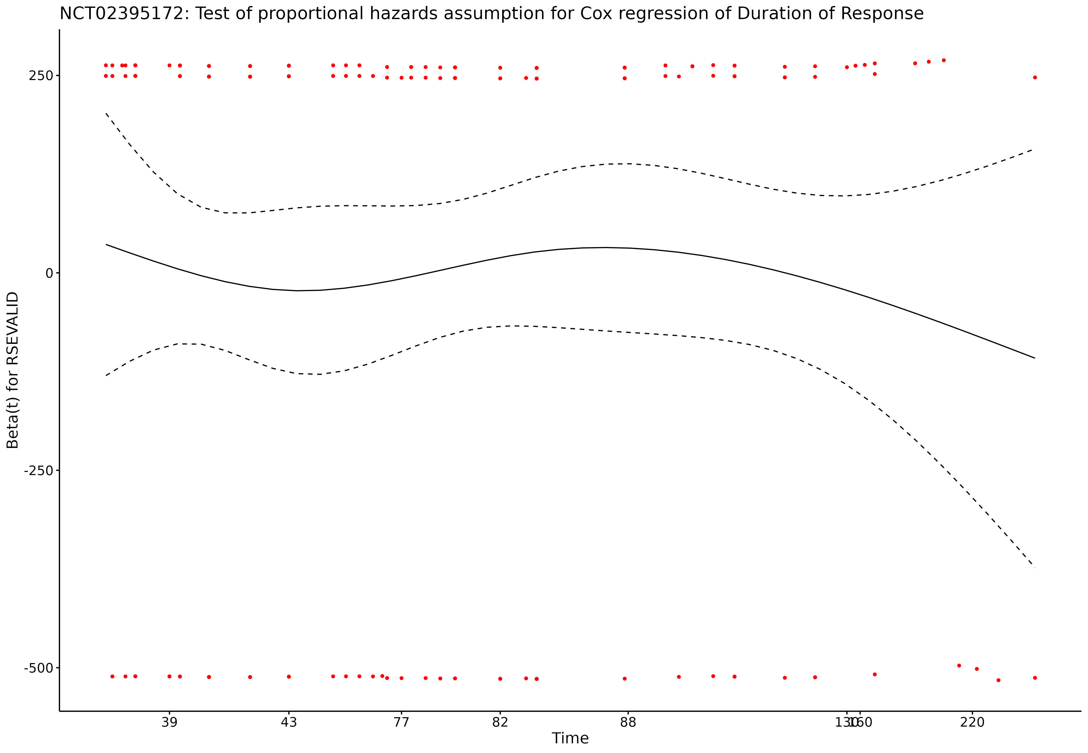
#| label: fig-dor-nct02395172-cox-zph
#| fig-cap: "Schoenfeld residuals for the Cox proportional hazards model for duration of response (DoR) for study NCT02395172."
#| fig-pos: 'H'
knitr::include_graphics(
"./images/survival_images/NCT02395172_dor_cox_zph.jpeg"
)
```
##### NCT03434379
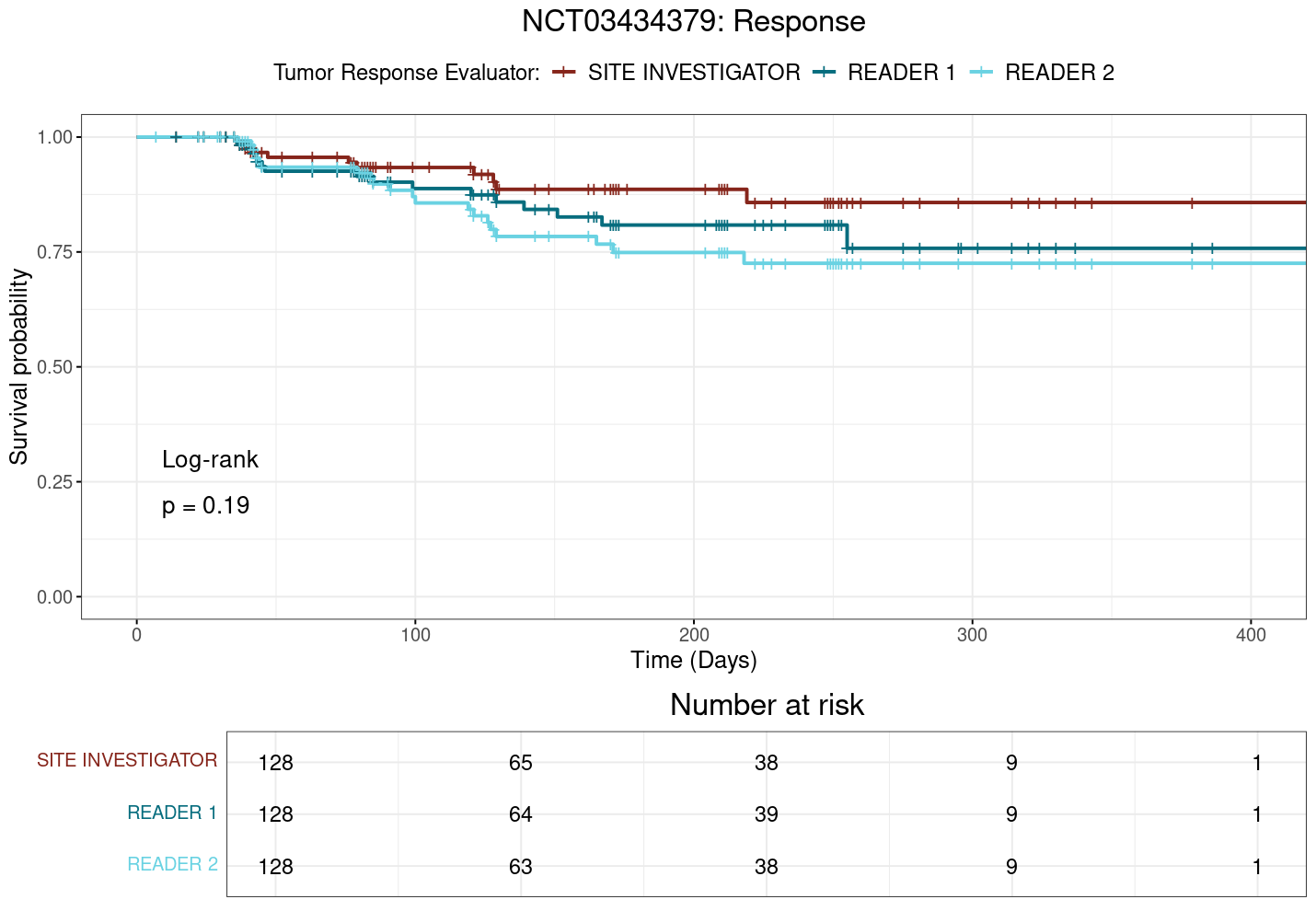
```{r}
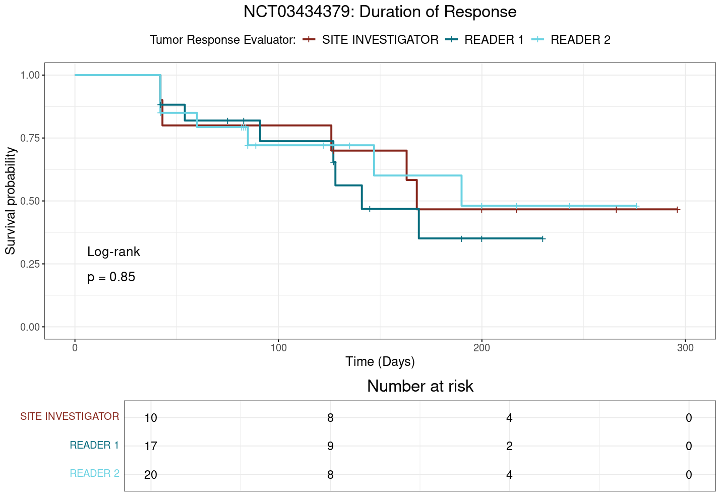
#| label: fig-dor-nct03434379-km
#| fig-cap: "Kaplan-Meier survival plot for duration of response (DoR) for study NCT03434379."
#| fig-pos: 'H'
knitr::include_graphics(
"./images/survival_images/NCT03434379_dor_kaplan_meier.png"
)
```
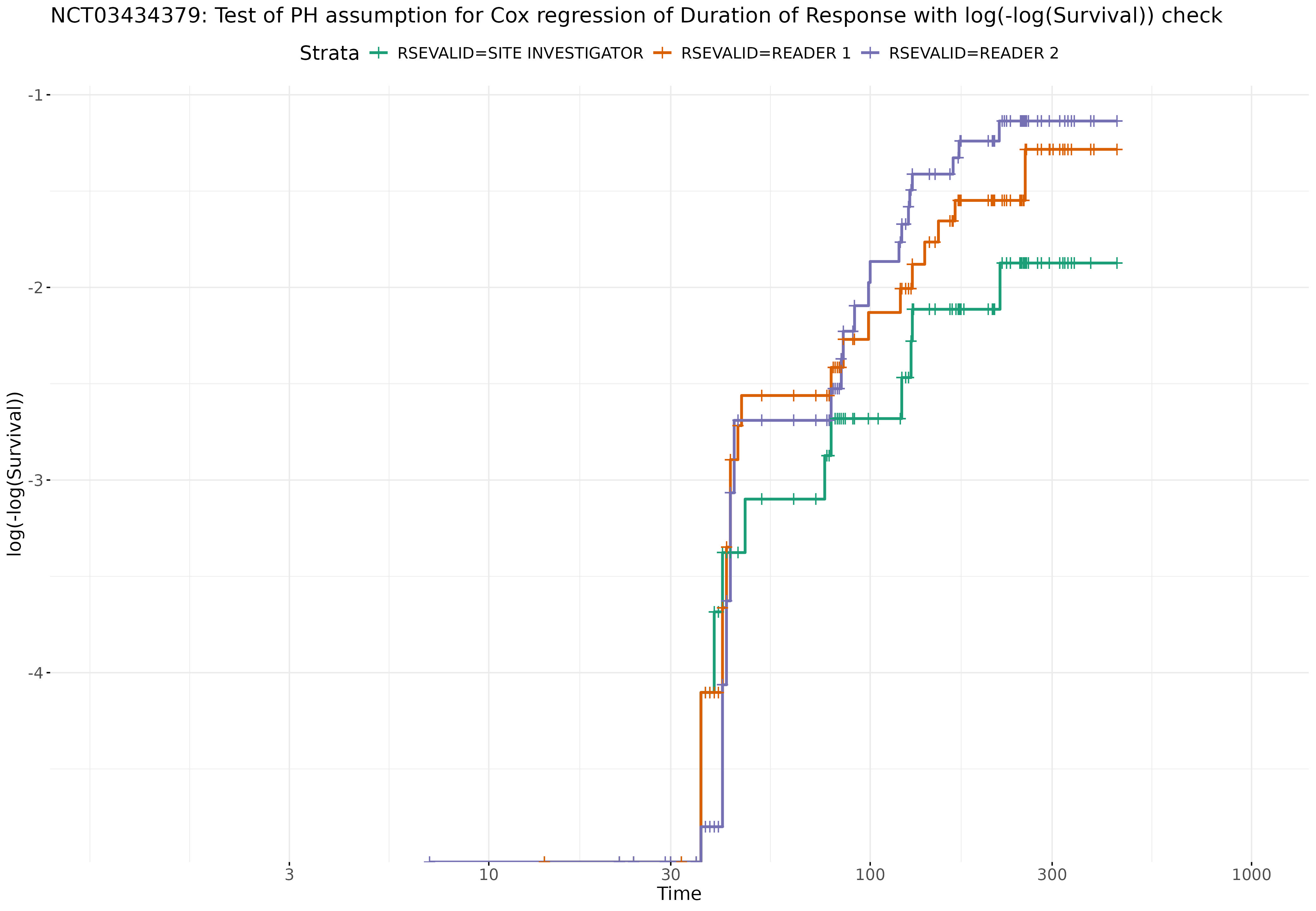
```{r}
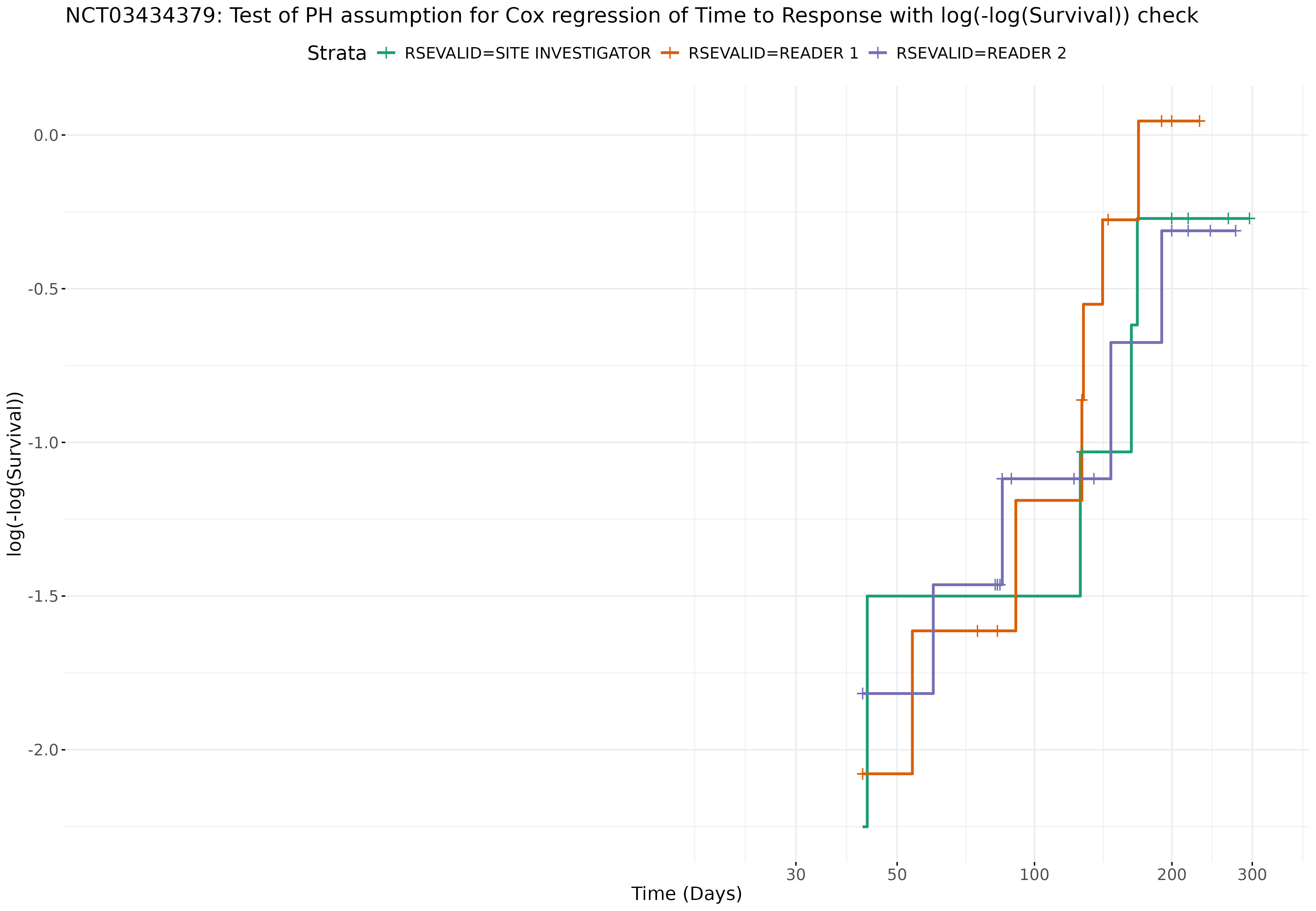
#| label: fig-dor-nct03434379-cloglog
#| fig-cap: "Log-minus-log survival plot for duration of response (DoR) for study NCT03434379."
#| fig-pos: 'H'
knitr::include_graphics(
"./images/survival_images/NCT03434379_dor_cox_cloglog.jpeg"
)
```
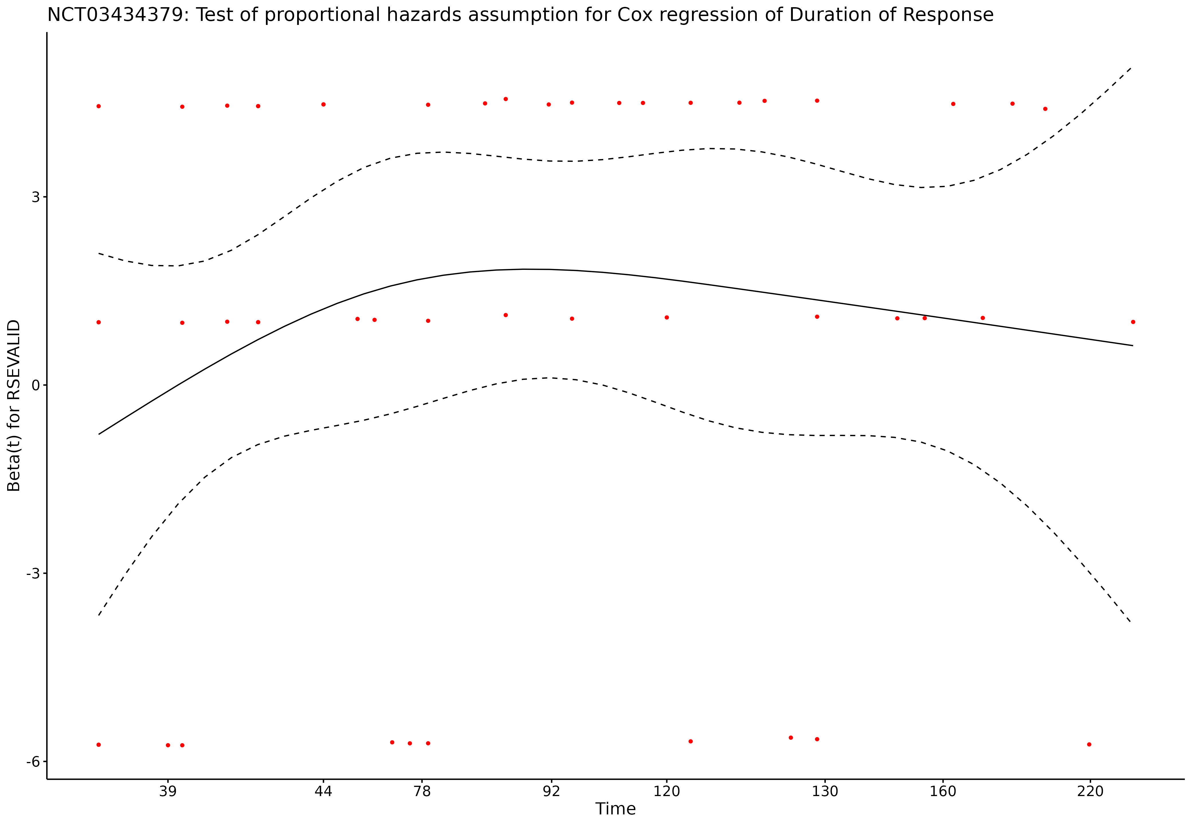
```{r}
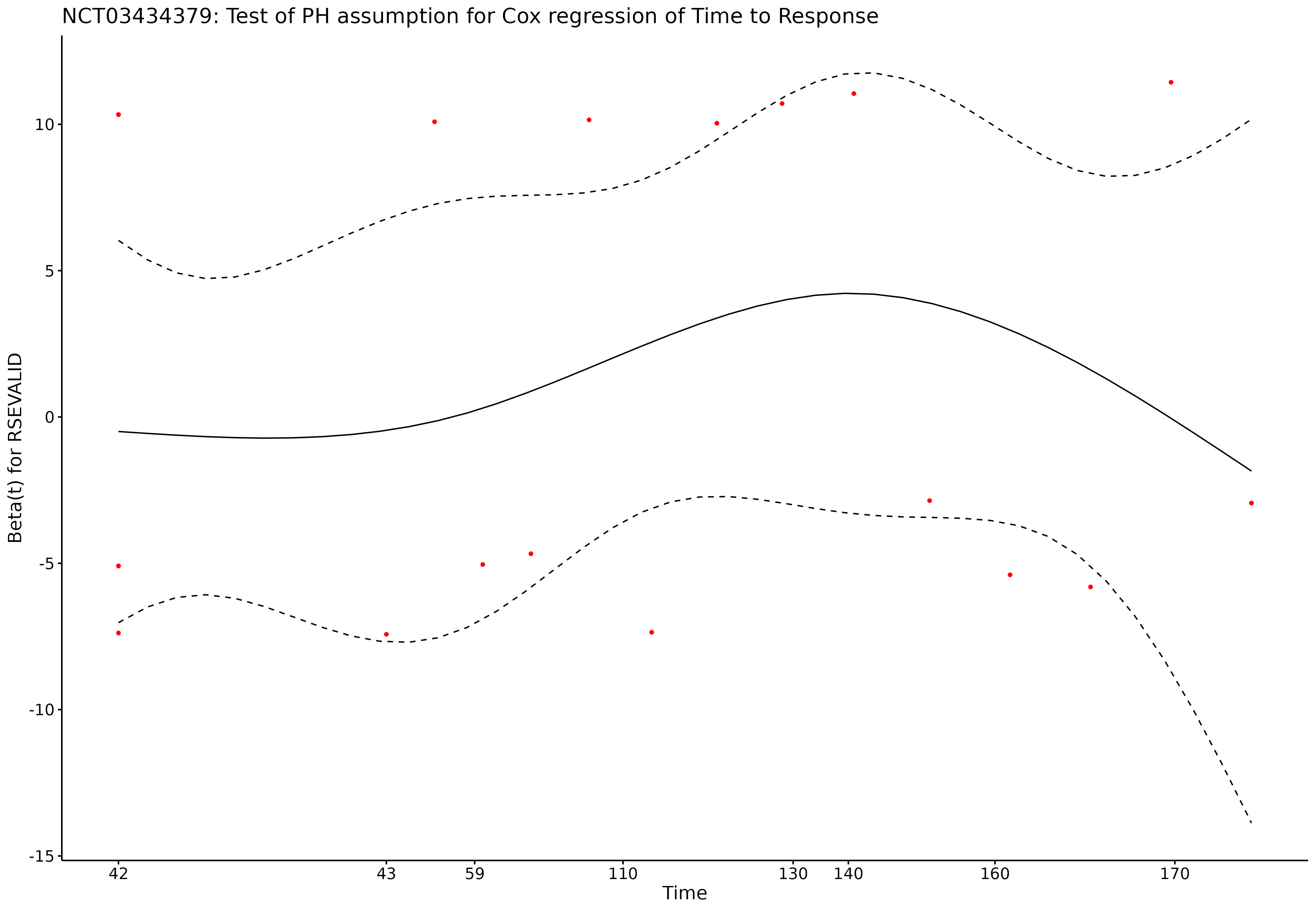
#| label: fig-dor-nct03434379-cox-zph
#| fig-cap: "Schoenfeld residuals for the Cox proportional hazards model for duration of response (DoR) for study NCT03434379."
#| fig-pos: 'H'
knitr::include_graphics(
"./images/survival_images/NCT03434379_dor_cox_zph.jpeg"
)
```
##### NCT03631706
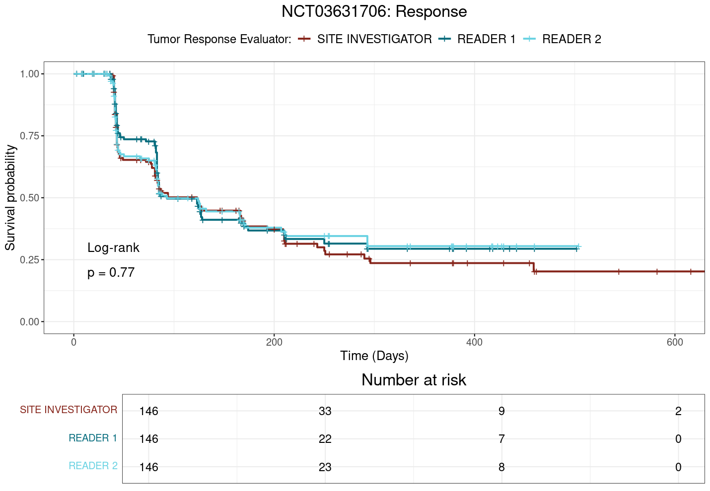
```{r}
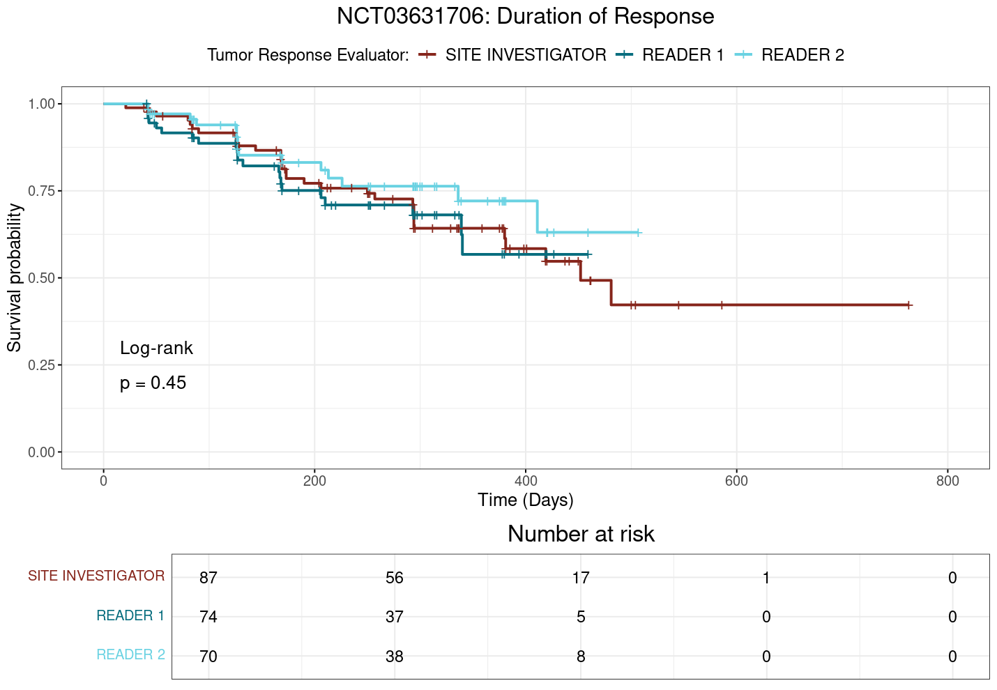
#| label: fig-dor-nct03631706-km
#| fig-cap: "Kaplan-Meier survival plot for duration of response (DoR) for study NCT03631706."
#| fig-pos: 'H'
#| out-width: "85%"
knitr::include_graphics(
"./images/survival_images/NCT03631706_dor_kaplan_meier.png"
)
```
```{r}
#| label: fig-dor-nct03631706-cloglog
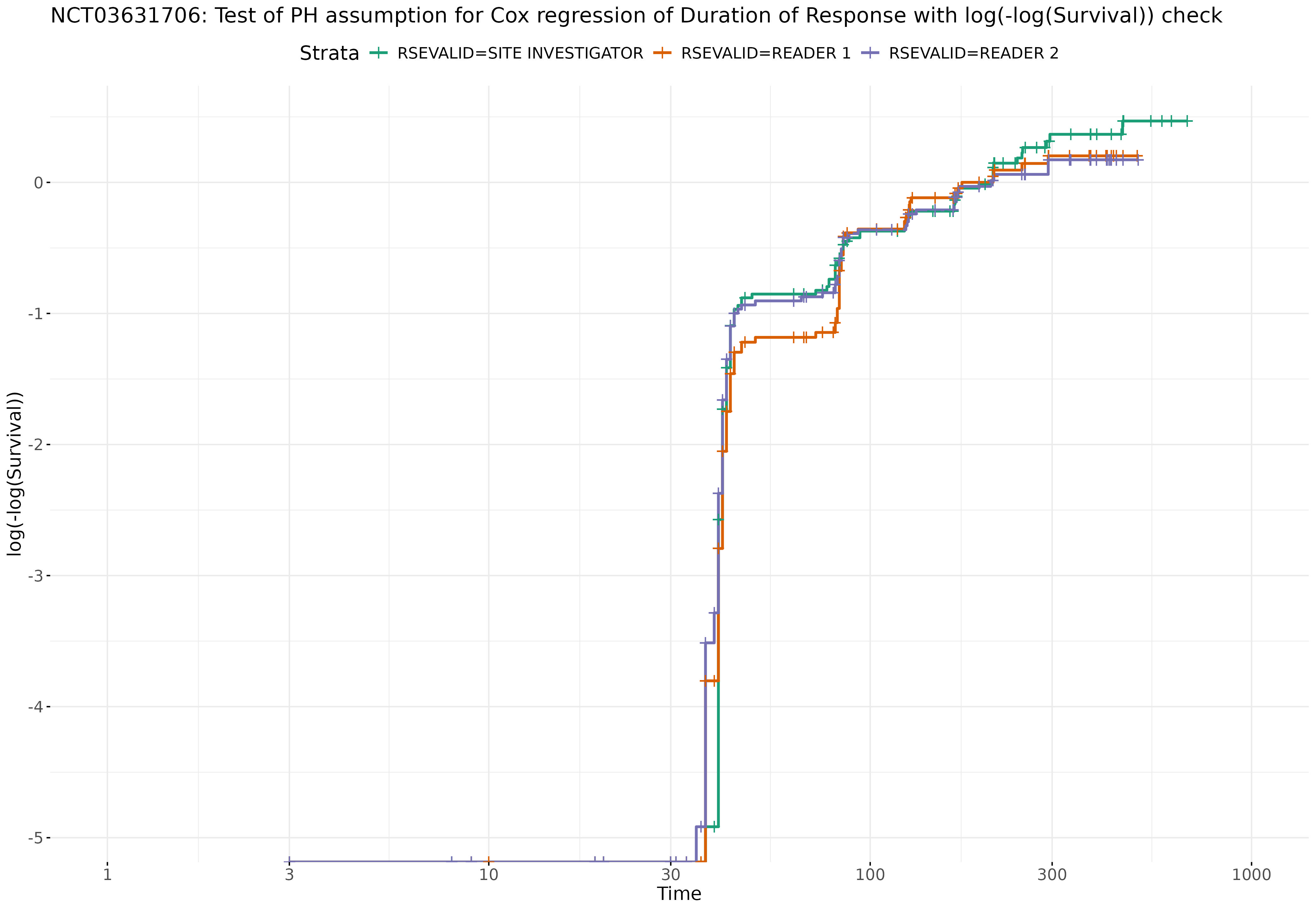
#| fig-cap: "Log-minus-log survival plot for duration of response (DoR) for study NCT03631706."
#| fig-pos: 'H'
#| out-width: "85%"
knitr::include_graphics(
"./images/survival_images/NCT03631706_dor_cox_cloglog.jpeg"
)
```
```{r}
#| label: fig-dor-nct03631706-cox-zph
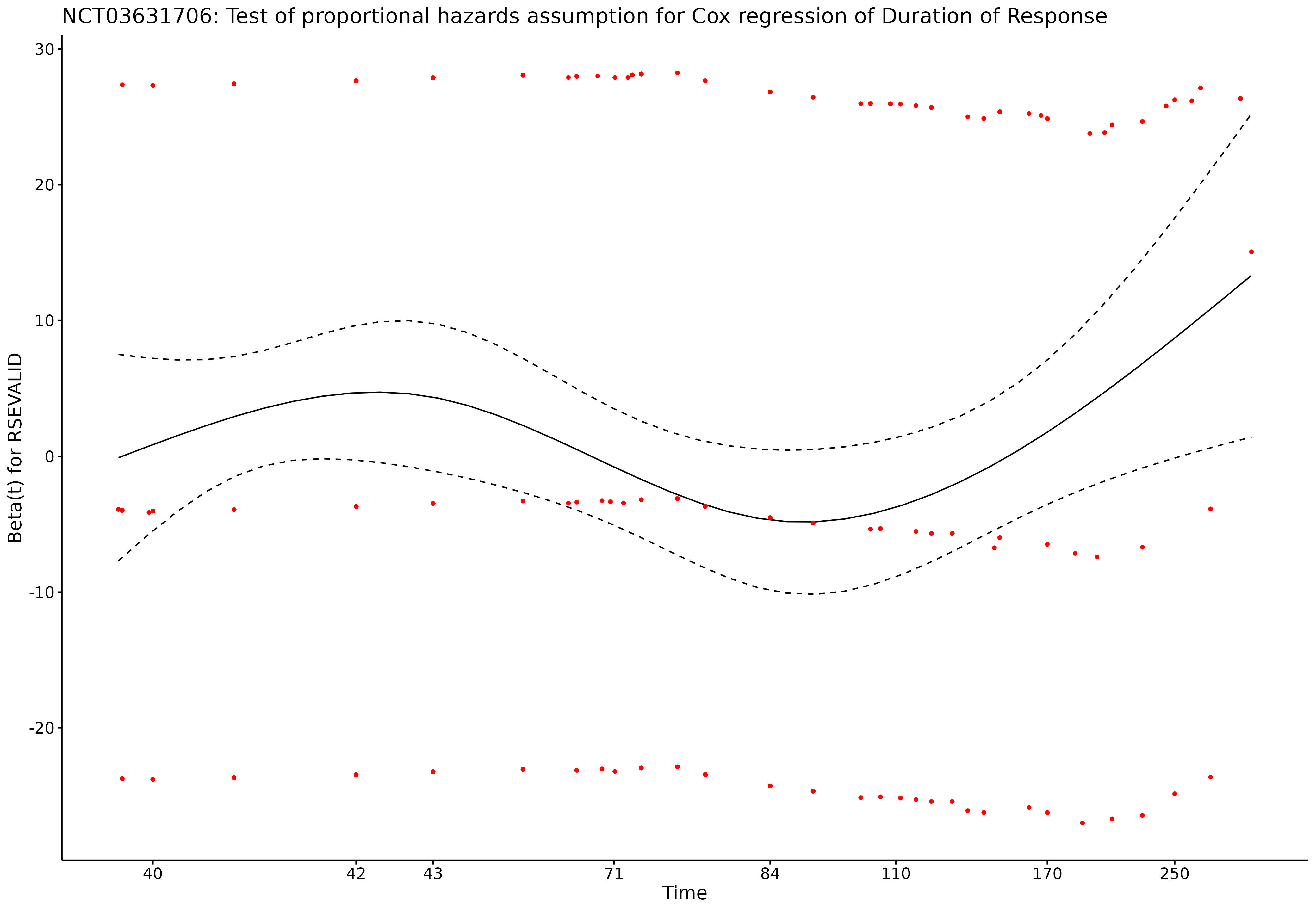
#| fig-cap: "Schoenfeld residuals for the Cox proportional hazards model for duration of response (DoR) for study NCT03631706."
#| fig-pos: 'H'
#| out-width: "85%"
knitr::include_graphics(
"./images/survival_images/NCT03631706_dor_cox_zph.jpeg"
)
```
### Time-to-Event Meta-Analyses
```{r}
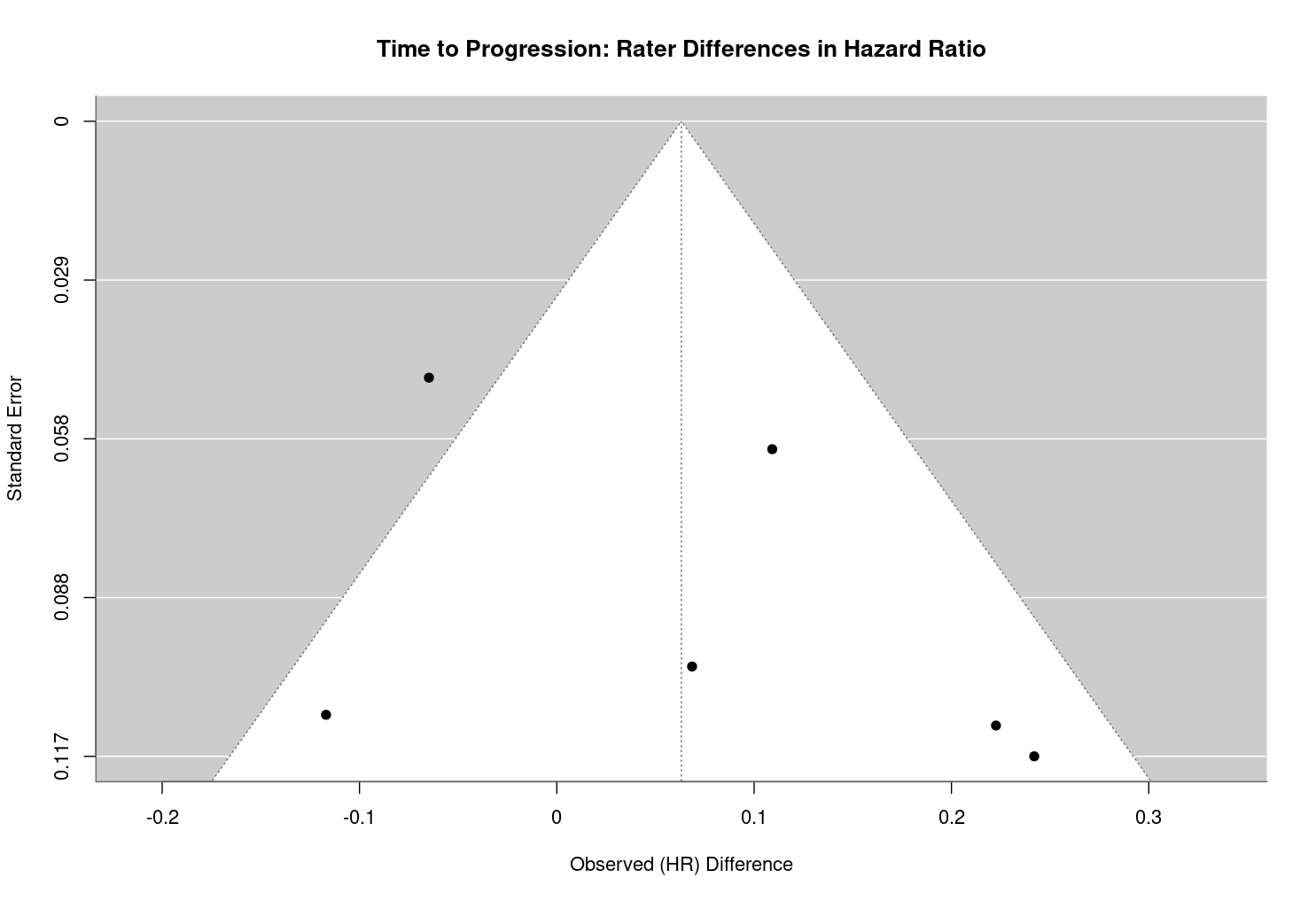
#| label: fig-ttp-hr-meta-analysis-forest-plot-repeat
#| fig-cap: "Forest plot of hazard ratios for TTP from the meta-analysis of time to event outcomes"
knitr::include_graphics(
"images/survival_images/progression_funnel_plot.png"
)
```
```{r}
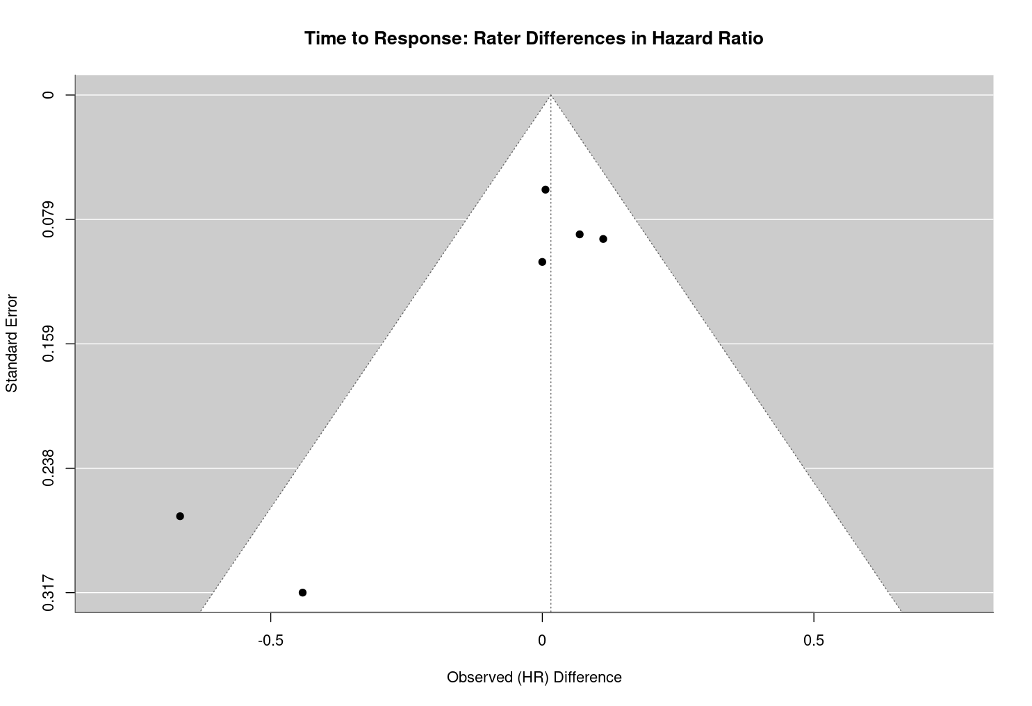
#| label: fig-ttr-hr-meta-analysis-funnel-plot
#| fig-cap: "Funnel plot of hazard ratios for TTR from the meta-analysis of time to event outcomes"
knitr::include_graphics(
"images/survival_images/response_funnel_plot.png"
)
```
```{r}
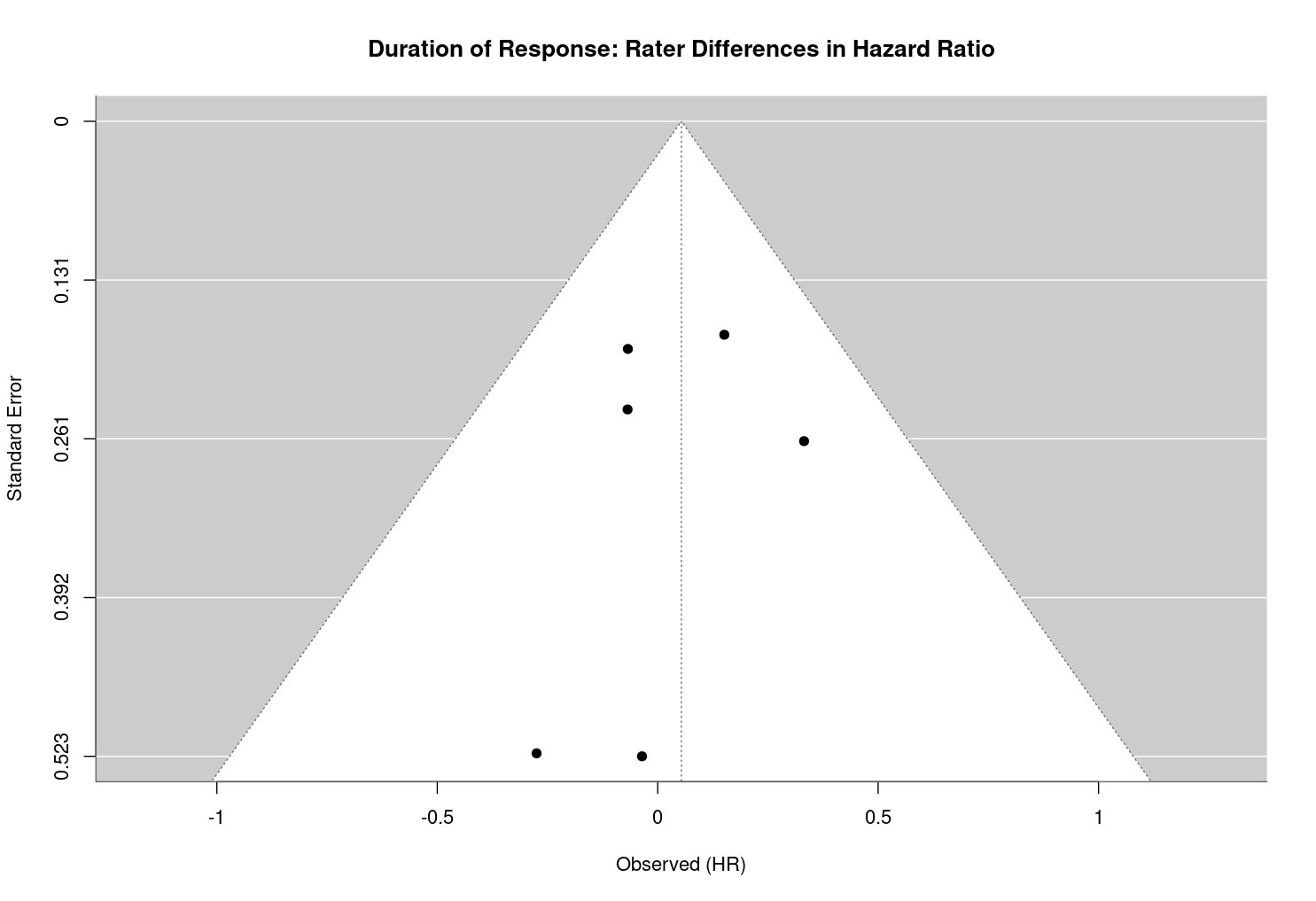
#| label: fig-dor-hr-meta-analysis-funnel-plot
#| fig-cap: "Funnel plot of hazard ratios for DOR from the meta-analysis of time to event outcomes"
knitr::include_graphics(
"images/survival_images/dor_funnel_plot.png"
)
```
\newpage
## Sensitivity Analyses
```{r}
source("data/simulations/plot_heatmaps.R")
source("data/simulations/irr/plot_irr_sims.R")
```
```{r}
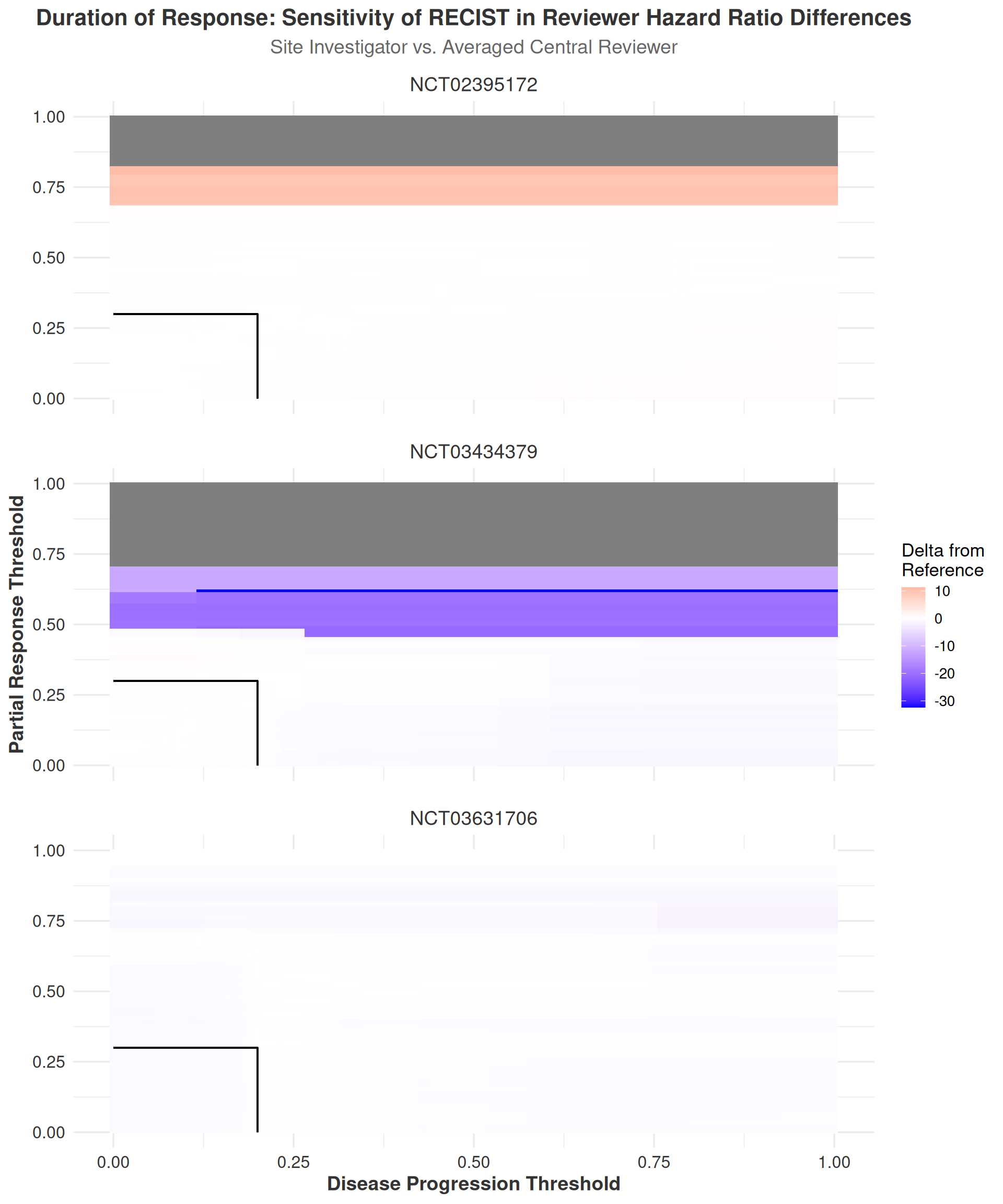
#| label: fig-heatmap-dor-unfiltered
#| fig-cap: "Heatmap of Change in Differences between Raters for DoR across RECIST thresholds, unfiltered data"
#| fig-height: 12
#| fig-width: 10
list.files("data/simulations/dor", full.names = T) %>%
grep("^(?!.*filtered).*\\.rds$", ., value = T, perl = TRUE) %>%
setNames(c("NCT02395172", "NCT03631706", "NCT03434379")) %>%
map(readRDS) %>%
bind_rows(.id = "Study") %>%
arrange(Study) %>%
plot_heatmaps(
x = progression_threshold,
y = partial_response_threshold,
fill = difference_from_actual,
wrapper = Study
) +
labs(
title = "Duration of Response: Sensitivity of RECIST in Reviewer Hazard Ratio Differences",
subtitle = "Site Investigator vs. Averaged Central Reviewer",
x = "Disease Progression Threshold",
y = "Partial Response Threshold",
fill = "Delta from\nReference"
)
```
```{r}
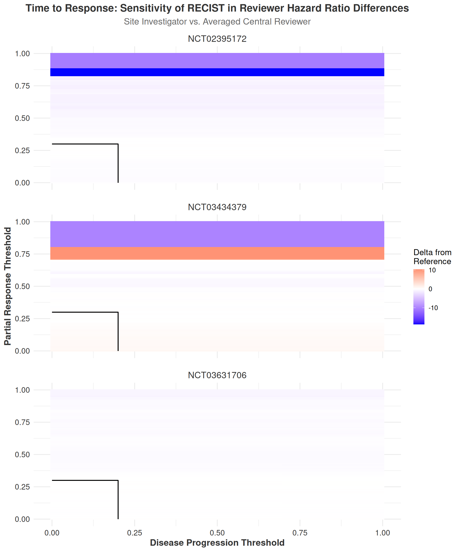
#| label: fig-heatmap-ttr-unfiltered
#| fig-cap: "Heatmap of Change in Differences between Raters for TTR across RECIST thresholds, unfiltered data"
#| fig-height: 12
#| fig-width: 10
list.files("data/simulations/response", full.names = T) %>%
grep("^(?!.*filtered).*\\.rds$", ., value = T, perl = TRUE) %>%
setNames(c("NCT02395172", "NCT03631706", "NCT03434379")) %>%
map(readRDS) %>%
bind_rows(.id = "Study") %>%
arrange(Study) %>%
plot_heatmaps(
x = progression_threshold,
y = partial_response_threshold,
fill = difference_from_actual,
wrapper = Study
) +
labs(
title = "Time to Response: Sensitivity of RECIST in Reviewer Hazard Ratio Differences",
subtitle = "Site Investigator vs. Averaged Central Reviewer",
x = "Disease Progression Threshold",
y = "Partial Response Threshold",
fill = "Delta from\nReference"
)
```