2 Methods and Materials
This section is broadly divided into two parts: the first part describes the data sources and how the data for this study are sourced, while the second part details the statistical analyses performed on the data. The methods and materials described here are designed to ensure transparency, reproducibility, and rigor in the research process, adhering to best practices in meta-analyses, and in scientific reporting more broadly.
2.1 Data Sources
Data for this study are sourced from two primary domains: a systematic review of the literature and proprietary data extracted from clinical trials. The literature review focuses on peer-reviewed studies reporting inter-rater reliability metrics for RECIST 1.1 assessments, while the clinical trial data are obtained from three specific trials that utilize RECIST 1.1 criteria for evaluating treatment responses made available through TransCelerate BioPharma Inc.’s DataCelerate™ platform (1,2). The trials are selected based on their use of RECIST 1.1 criteria, the availability of assessments from both site investigators and central reviewers, and the inclusion of data on target lesions, non-target lesions, new lesions, and SLD measurements. Details for both data sources are provided below.
2.1.1 Literature Search
A systematic search of the literature is undertaken to identify peer-reviewed studies that report inter-rater reliability metrics for assessments conducted using RECIST 1.1. The search is designed to comprehensively capture studies that quantitatively evaluate the degree of agreement between multiple independent raters, employing established statistical measures of inter-rater reliability.
2.1.1.1 Search Strategy & Study Eligibility
The primary search was conducted in the PubMed/MEDLINE database using a combination of Medical Subject Headings (MeSH) and free-text terms (3). The search strategy encompasses two core conceptual domains: employment of RECIST criteria in the study and inter-rater reliability. Searches were conducted with Essie syntax to optimize sensitivity to identifying relevant studies (4). The search terms included combinations of expressions including “RECIST inter-rater reliability”, “(RECIST OR Response Evaluation Criteria in Solid Tumors)”, and “(Cohen’s kappa OR Fleiss’ kappa OR kappa)”
In addition to the primary search, targeted supplementary searches were carried out to further enhance the comprehensiveness of the review and capture potentially relevant studies not indexed in PubMed. A supplementary search of Google Scholar was performed using the keywords “RECIST interrater reliability”, and the first 50 results retrieved were screened for eligibility, with attention to studies published in non-MEDLINE indexed journals.
Eligibility criteria were defined a priori to ensure the systematic and unbiased inclusion of relevant studies. To be included, studies must be published in peer-reviewed journals, report quantitative inter-rater reliability statistics for RECIST 1.1 assessments (either Cohen’s \(\kappa\) or Fleiss’ \(\kappa\)), and involve two or more independent qualified raters (i.e. medical doctors) evaluating identical imaging datasets. Only studies that provide sufficient methodological detail to enable data extraction and critical appraisal were considered. Furthermore, only articles published in English and after the introduction of RECIST 1.1 in 2009 are eligible (5).
Studies were excluded if they employ the outdated RECIST 1.0 criteria, if they employ variants of RECIST such as mRECIST (6) and iRECIST (7), if they report only descriptive rather than statistical measures of agreement, and if they only provide continuous measures of inter-rater reliability such as intra-class correlation coefficients. In addition, studies lacking sufficient detail regarding statistical methodology or reliability calculation procedures, studies not reporting inter-rater reliability metrics, and duplicated studies are all excluded.
2.1.1.2 Study Screening and Selection Process
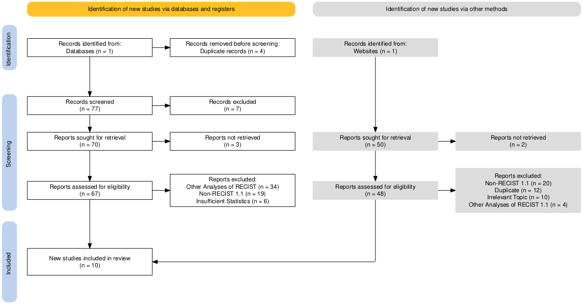
To ensure transparency and reproducibility in the identification, screening, and selection of studies, we follow the Preferred Reporting Items for Systematic Reviews and Meta-Analyses (PRISMA) 2020 guidelines (8). The study selection process is documented using a PRISMA flow diagram, which details the number of records identified, screened, assessed for eligibility, and included in the final analysis, as well as the reasons for exclusion at each stage. This approach provides a standardized and rigorous framework for reporting systematic reviews and meta-analyses.
All searches were conducted between April 1 and April 2, 2025. The study selection process was carried out in two stages to minimize bias and ensure comprehensive identification of eligible studies. In the first stage, titles and abstracts of all retrieved records were independently screened by PC to determine potential eligibility. Records that clearly meet inclusion criteria (i.e. because \(\kappa\) is reported in the article abstract) or whose eligibility cannot be determined based on the abstract alone were retained for full-text evaluation.
In the second stage, the full texts of potentially eligible studies were assessed in detail against the predefined inclusion and exclusion criteria. Studies that meet all inclusion criteria were incorporated into the final dataset. In addition to database searching, the reference lists of all included studies were manually reviewed to identify any additional relevant articles not captured by the primary or supplementary search strategies. The entire study selection process was documented and reported in Figure 2.1 in accordance with the PRISMA guidelines to ensure transparency and reproducibility. The diagram was produced using the {PRISMA}1 R Package (9).
2.1.1.3 Data Extraction
For data extraction, we used a standardized form developed specifically for the purposes of this review. Extracted study characteristics include bibliographic information (author, year, and database), number of raters, the type of inter-rater reliability statistic reported (Cohen’s \(\kappa\) or Fleiss’ \(\kappa\)), the estimate for the reported statistic, and the corresponding standard error or confidence interval. The context in which the study is conducted (e.g. clinical trial, retrospective study, etc.) was also collected, and summarized as either being a Clinical Trial or Other Study as the only major distinction of relevance for this paper is whether or not the study data is derived from a clinical trial. The term “Other Study” is chosen to describe the remaining studies as they are done in a mix of prospective (10–12) and retrospective (13–19) designs across 1 to 3 sites, but such study design elements are not otherwise of significance to this review.
When studies fail to directly report sufficient details of their inter-rater reliability statistics, namely the standard error of the estimate, these values are derived from the reported 95% confidence intervals using standard statistical formulas. Studies that neither report confidence intervals nor standard errors are necessarily excluded from the meta-analyses.
2.1.2 Trial Data
Potential clinical trials were identified by querying the ClinicalTrials.gov API v2.0.3 “studies” endpoint (20), specifically targeting the query.outc field, which allows searching for both primary and secondary outcome measures. This field was queried using Essie syntax (21) for the string: “RECIST OR response evaluation criteria in solid tumors OR sum of longest diameters OR SLD”, to identify studies that directly or indirectly referenced RECIST criteria in their primary or secondary outcomes. We did not restrict the search criteria to strictly “RECIST” or “response evaluation criteria in solid tumors” because it was noted in preliminary searches that some studies only referenced the terms “sum of longest diameters” and “SLD” while implicitly using the RECIST rating criteria.
Studies identified via querying the ClinicalTrials.gov API were then cross-referenced with those available through TransCelerate BioPharma Inc.’s DataCelerate™ platform. TransCelerate is a non-profit organization promoting collaboration across biopharmaceutical companies, with approximately 20 major pharmaceutical partner companies (22). The DataCelerate™ platform in particular aims to facilitate the sharing of high-quality historical trial data (HTD) across companies in a manner compliant with U.S. Code of Federal Regulations privacy laws as well as adhering to other globally relevant data privacy laws (2); in other terms, it provides a secure, standardized environment ensuring regulatory compliance and protects patient confidentiality while enabling collaborative research and secondary analyses across the pharmaceutical industry. Of note, the data available for this project via DataCelerate™ is exclusively placebo group/standard of care (PSOC) data, also commonly referred to as “control group” data (2).
The subset of studies identified by cross-referencing results from ClinicalTrials.gov against DataCelerate™ undergo manual review to confirm the use of RECIST 1.1 criteria, the availability of RECIST assessments from both site investigators and central reviewers, and the inclusion of data on target lesions, non-target lesions, new lesions, and SLD measurements. Three trials meet all inclusion criteria: NCT02395172, NCT03434379, and NCT03631706. Two of these trials investigate treatments for non-small cell lung cancer, while the third focuses on hepatocellular carcinoma. Detailed trial characteristics are summarized in Table 2.1.
| Trial ID | NCT02395172 | NCT03434379 | NCT03631706 |
|---|---|---|---|
| Cancer | Non-Small Cell Lung Cancer | Hepatocellular Carcinoma | Non-Small Cell Lung Cancer |
| Label | Open | Open | Open |
| Phase | Phase 3 | Phase 3 | Phase 3 |
| Control Group Size | n=329 | n=128 | n=146 |
| Control Group Treatment | Docetaxel (cytotoxic) | Sorafenib (targeted cytostatic) | Pembrolizumab (immunotherapy) |
| Population Notes | NSLCC patients what have progressed disease | Advanced or metastatic HCC patients | NSLCC patients |
| Locations | 260 international sites | 119 international sites | 119 international sites |
The therapeutic agents in these trials represent three distinct mechanisms of action: cytotoxic treatments that induce cell death primarily through chemotherapy (23), cytostatic agents that inhibit cell division (23), and immunotherapies that activate targeted immune responses (24). This distinction is methodologically significant as these different modalities produce distinct response patterns that may affect RECIST assessment validity. For example, immunotherapies can cause pseudoprogression due to immune cell infiltration before actual tumor response occurs, potentially leading to misclassification under standard RECIST criteria (25).
For each clinical trial, data are structured in accordance with the Study Data Tabulation Model (SDTM) as defined by the Clinical Data Interchange Standards Consortium (CDISC) (26). The data standards developed by CDISC ensure consistency and regulatory compliance in the submission of clinical trial data, and also helps facilitate interoperability and data analyses within and across institutions analyzing trial data. Specifically, the tumor (TU), tumor results (TR), and disease response (RS) domains are employed to capture and organize data related to tumor assessments and treatment responses.
The TU domain is used to uniquely identify tumors and lesions, specifically their classification as target, non-target, or new lesions, as per RECIST 1.1 guidelines (27). The TR domain records quantitative and qualitative measurements of these identified tumors, such as size and progression status, which are essential for calculating the SLD and assessing changes over time (27). The RS domain captures the overall response evaluations (e.g., complete response, partial response, stable disease, or progressive disease) based on the RECIST criteria (28), and is largely derived from the TU and TR domains. These domains work in concert to provide a comprehensive and traceable representation of tumor burden through monitoring of individual tumors and the SLD of those tumors, as well as treatment efficacy by way of deriving outcomes according to the RECIST criteria (29).
Data extracted and/or derived from the TU, TR, and RS SDTM domains include SLD measurements and RECIST 1.1 assessments for overall response, target lesions, non-target lesions, and new lesions. These data are available at scheduled imaging time points as defined by each study protocol. At each of these time points, imaging assessments are independently performed by three raters: one on-site investigator and two central reviewers.
2.2 Statistical Analyses
The statistical analyses are divided into three major sections reflecting the three main lines of enquiry of this thesis. First, the procedures for the IRR meta-analyses are covered including a review of Cohen’s and Fleiss’ \(\kappa\), the mathematical bases for transforming the IRR data, and details of how the meta-analyses are conducted and interpreted. Second, we present a multi-part analysis of differences between site investigators and central reviewers for the trial endpoints ORR, TTP, TTR, and DoR. Finally, this chapter concludes by describing the sensitivity analysis which aims to elucidate whether differences between site investigators and central reviewers in trial outcome measures has a dependency on the disease progression and response thresholds defined by RECIST. A helpful framing question to keep in mind while reading the methods and results for the sensitivity analyses is as follows: “if we change the response and progression thresholds, how much more or less do the site investigators and central reviewers agree with one another?”
2.2.1 Inter-Rater Reliability Meta-Analysis
A meta-analysis is a statistical technique that combines the results of multiple independent studies to produce a single summary estimate of an effect or association (30). By synthesizing data across studies, meta-analyses increase statistical power, improve estimates of effect size, and help identify patterns or sources of heterogeneity that may not be apparent in individual studies (30). This approach is especially valuable in fields where individual studies may be small or yield conflicting results, as it provides a more comprehensive and objective assessment of the evidence. Meta-analyses typically employ either fixed-effect or random-effects models, with the former assuming that all studies estimate the same underlying effect size, while the latter allows for variability between studies in terms of populations, methodologies, and other factors (30). The choice of model depends on the research question, the degree of heterogeneity among studies, and the assumptions about the data.
As such we conducted a series of random-effects meta-analyses focusing on inter-rater reliability (IRR) statistics in order to evaluate the consistency of RECIST 1.1 assessments across different raters of the same data. Specifically, we analyzed Cohen’s \(\kappa\), Fleiss’ \(\kappa\), and a combined set of both measures, with all analyses restricted to the Overall RECIST 1.1 Outcome, which was generally the only available endpoint across the studies identified in the literature search.
2.2.1.1 IRR Measures Review: Cohen’s and Fleiss’ \(\kappa\)
Cohen’s kappa (\(\kappa\)) is a statistical measure assessing the degree of agreement between two raters/observers who each classify the same items. Unlike a simple percentage agreement measure, Cohen’s \(\kappa\) accounts for agreement between raters that occurs by chance alone which provides a more robust measurement of rater agreement (31). The calculation of Cohen’s \(\kappa\) is given by (31):
\[ \kappa = \frac{p_o - p_e}{1 - p_e} \tag{2.1}\]
where
\[ p_o = \sum_{i=1}^k p_{ii} \tag{2.2}\]
is the observed proportion of agreement and \(p_{ii}\) denotes the proportion of items for which both raters independently assigned category \(i\), and \(k\) is the total number of categories. Likewise,
\[ p_e = \sum_{i=1}^k p_{iA} \cdot p_{iB} \tag{2.3}\]
is the expected proportion of agreement by chance, with \(p_{iA}\) is the proportion of items that rater A assigns to category \(i\), \(p_{iB}\) is the proportion of items that rater B assigns to category \(i\), and \(k\) is the number of categories.
Interpretation of the corresponding values is relatively straightforward as \(\kappa\) is mathematically bounded on the interval \([-1,1]\) with positive values indicating rater agreement and negative values indicating disagreement (32). However, observed values are typically assumed to be on the range \((0,1]\) as this is the range in which raters show partial agreement up until perfect agreement at \(\kappa=1\) (32). Approximate qualitative interpretations of values on this range have been proposed by Landis et al. (33), and are reproduced in Table 2.2 below.
| Kappa | Interpretation |
|---|---|
| <0.00 | Poor agreement |
| 0.00-0.20 | Slight agreement |
| 0.21-0.40 | Fair agreement |
| 0.41-0.60 | Moderate agreement |
| 0.61-0.80 | Substantial agreement |
| 0.81-1.00 | Almost perfect agreement |
While Table 2.2 provides a useful framework for interpreting Cohen’s \(\kappa\) values, it is important to note that these benchmarks are arbitrary and may not apply universally across all contexts. The interpretation of \(\kappa\) values can vary depending on the specific application, the nature of the data, and the clinical or research context in which the ratings are made. Therefore, while these benchmarks provide a general guideline and serve as the starting point for discussions around the IRR in this paper, they must be applied with caution and in conjunction with other contextual factors.
As with other statistical measures, the interpretation of Cohen’s \(\kappa\) should likewise be informed by the variability of the data (i.e. confidence intervals and standard errors) and the specific clinical or research context in which it is applied. In some cases, reviewing the marginal distributions of the data may provide additional insights into the nature of the source of (dis-)agreement between raters.
An important limitation of Cohen’s \(\kappa\) is its sensitivity to the strictness of category definitions, particularly when categories are conceptually similar or adjacent in clinical meaning. In the context of RECIST 1.1, for example, a complete response (CR) and a partial response (PR) are treated as distinct categories, even though both represent favorable treatment outcomes, as will be explored in our analyses of objective response rate. Because \(\kappa\) penalizes all disagreements equally, however, it does not account for the practical or clinical proximity of such categories. As a result, disagreements between raters that involve adjacent or similar categories can disproportionately lower the \(\kappa\) value, even if the distinction is of limited clinical impact. This limitation should be considered when interpreting \(\kappa\) values in settings where the boundaries between categories may be somewhat arbitrary or where minor disagreements do not necessarily reflect meaningful differences in clinical judgment.
In addition to advocating for caution in interpreting Cohen’s \(\kappa\) values, it is also important to note that the statistic is only applicable for assessing agreement between two raters. When more than two raters are involved, Fleiss’ \(\kappa\) is typically employed as an extension of Cohen’s \(\kappa\) that allows for the assessment of agreement among multiple raters simultaneously (34). Fleiss’ \(\kappa\) is calculated using a similar formula to Cohen’s \(\kappa\) that calculates an average agreement between raters while adjusting for expected agreement, and the yielded values are also on the range, \([-1,1]\) (34).
2.2.1.2 Compiling Inter-Rater Reliability Estimates
Estimates of Cohen’s and Fleiss’ \(\kappa\) statistics and their corresponding standard errors were extracted directly from the included studies when available. When standard errors were not reported, they were derived from the reported confidence intervals using standard statistical formulas assuming a normal distribution and a 95% confidence level. Specifically, the standard error (SE) was calculated as:
\[ SE = \frac{CI_{upper} - CI_{lower}}{2 \cdot Z_{0.975}} \tag{2.4}\]
where \(CI_{upper}\) and \(CI_{lower}\) are the upper and lower bounds of the confidence interval, respectively, and \(Z_{0.975}\) is the critical value from the standard normal distribution corresponding to a 95% confidence level (approximately 1.96).
To supplement the literature-based estimates, Fleiss’ \(\kappa\) was also calculated for the RECIST Overall outcome using data from the control arm data of the three clinical trials described previously. A standard R implementation for calculating the standard error (\(SE\)) of Fleiss’ \(\kappa\) could not be readily located2, and recent research has shown variance calculations for Fleiss’ \(\kappa\) that are derived from the variance calculates for Cohen’s \(\kappa\) (34) may be inappropriate for constructing confidence intervals (35). Rather than seek out a package implementing a potentially incorrect calculation of the \(SE\) of Fleiss’ \(\kappa\), \(SE\) values for these trial-based estimates were obtained via non-parametric bootstrapping with 10,000 resamples. All IRR calculations for the clinical trial data were performed using the {irr} package in R (36).
2.2.1.3 Logit Transformation of Kappa Values
A log transformation is frequently applied to effect size estimates in meta-analyses to (37), particularly for measures such as odds ratios, risk ratios, and hazard ratios. The primary rationale is that these effect sizes are inherently positive and often exhibit right-skewed distributions. Applying the natural logarithm (\(\ln\)) to these values thus serves several purposes: it stabilizes the variance, normalizes the distribution, and converts multiplicative relationships into additive ones (37), which simplifies statistical modeling and interpretation. On the log scale, confidence intervals are more likely to be symmetric, and the assumption of normality underlying many meta-analytic methods is better satisfied.
However, log transformation is not universally appropriate. It cannot be applied to effect sizes that can take negative values or are bounded (such as correlation coefficients or \(\kappa\) statistics), as the transformation may yield values outside the theoretical range or introduce interpretational difficulties. Additionally, back-transforming results to the original scale can sometimes complicate interpretation, especially for non-statistical audiences. In the case of Cohen’s and Fleiss’ \(\kappa\), which are both bounded on the range \([-1, 1]\), a special case of the log-transformation, the logit, was applied to obtain many of the same benefits seen in a log transformation, including stabilizing variance and ensuring that confidence intervals remained within the theoretical bounds of the statistic. The transformation was defined as:
\[ \text{logit}(\kappa) = \log\left(\frac{\kappa + 1}{1 - \kappa}\right) \tag{2.5}\]
The logit transformation is particularly well-suited for \(\kappa\) statistics because direct application of a standard logarithmic transformation is not possible for values that can be negative or zero, nor does it preserve the bounded nature of the statistic (38). The logit function maps the interval \((-1, 1)\) onto the entire real line, removing the bounds and allowing for the use of statistical methods that assume unbounded, normally distributed variables. Perhaps most importantly in the context of performing meta-analyses, this transformation ensures that confidence intervals, when back-transformed, remain within the theoretical limits of the \(\kappa\) statistic. As a result, the logit transformation enables more accurate and interpretable meta-analytic inference for bounded agreement measures.
To estimate the standard error of the logit-transformed kappa, the delta method was used (39). In simple terms, the delta method provides a way to estimate the standard error of a transformed statistic by using the standard error of the original statistic and the slope (derivative) of the transformation (40). It works by approximating how much uncertainty in the original value “carries over” after applying a mathematical function, such as the logit. This allows us to calculate confidence intervals for transformed values, even when the transformation is non-linear (40). Our approach is similar to Carpentier et al.(38) who applied such a transformation to Cohen’s \(\kappa\) data, but they assumed bounding of \(\kappa\) from 0 to 1. We followed the same approach, but with the more general bounding of \([-1, 1]\) to account for the fact that \(\kappa\) can take negative values, and our steps were informed by Muche et al. (40).
If \(\hat{\theta}\) is an estimator of a parameter \(\theta\) and \(g(\cdot)\) is a differentiable function, then:
\[ \text{Var}(g(\hat{\theta})) \approx \left(g'(\theta)\right)^2 \cdot \text{Var}(\hat{\theta}) \tag{2.6}\]
In our case, we are ultimately interested in the standard error of the logit-transformed \(\kappa\) estimate, which can be obtained by simply taking the square root of the variance:
\[ \text{SE}[g(\hat{\theta})] \approx |g'(\theta)| \cdot \text{SE}(\hat{\theta}) \tag{2.7}\]
The derivative of the logit transformation is given by:
\[ \begin{aligned} g'(\kappa) &= \frac{d}{d\kappa} \log\left(\frac{\kappa + 1}{1 - \kappa}\right) \\ &= \frac{d}{d\kappa} \left[ \log(\kappa + 1) - \log(1 - \kappa) \right] \\ &= \frac{1}{\kappa + 1} + \frac{1}{1 - \kappa} \\ &= \frac{(1 - \kappa) + (\kappa + 1)}{(\kappa + 1)(1 - \kappa)} \\ &= \frac{2}{1 - \kappa^2} \end{aligned} \tag{2.8}\]
Substituting this into the equation for the standard error of the logit-transformed \(\kappa\) gives us:
\[ \text{SE}[g(\hat{\theta})] = \frac{2}{1 - \kappa^2} \cdot \text{SE}(\hat{\theta}) \tag{2.9}\]
And replacing \(\text{SE}(\hat{\theta})\) with \(SE_{\kappa}\), the standard error of the original \(\kappa\) estimate, we obtain the final formula for the standard error of the logit-transformed \(\kappa\):
\[ SE_{\text{logit}(\kappa)} = \frac{2 \cdot SE_{\kappa}}{1 - \kappa^2} \tag{2.10}\]
where \(SE_{\kappa}\) is the standard error of the original \(\kappa\) estimate and \(\kappa\) is the original \(\kappa\) estimate. This is the transformation applied to all \(\kappa\) estimates prior to conducting the meta-analyses, and the back-transformation is applied to the pooled estimates and confidence intervals after fitting the random-effects model.
2.2.1.4 Meta-Analysis Procedure
For each set of \(\kappa\) estimates (Cohen’s, Fleiss’ and the combined set), meta-analyses were performed on the logit-transformed values to ensure that pooled estimates and confidence intervals remained within the theoretical bounds of the statistic. The logit transformation was applied to each study’s \(\kappa\) value using Equation 2.5 and its standard error using Equation 2.10, as described above. Meta-analyses were conducted using a random-effects model, which accounts for both within-study and between-study variability. This approach is appropriate given the expected heterogeneity in study populations, imaging protocols, and assessment procedures across the included studies. The estimate of the average effect from a random-effects analysis will be more conservative than that of a fixed-effect analysis, but provides a more appropriate, generalizable result given the heterogeneity of the included studies.
The random-effects model was implemented using the rma() function from the {metafor} package in R (41), specifying the Restricted Maximum Likelihood (REML) estimator to estimate the between-study variance (\(\tau^2\)). Each study’s contribution to the pooled estimate was weighted by the inverse of its total variance (the sum of within-study and between-study variance components). After fitting the model, pooled logit-transformed estimates and their confidence intervals were back-transformed to the original \(\kappa\) scale using the inverse logit function:
\[ \kappa = \frac{e^x - 1}{e^x + 1} \tag{2.11}\]
Heterogeneity among studies was assessed using the \(I^2\) statistic and Cochran’s \(Q\) test, both of which are standard outputs of the {metafor} package. The \(I^2\) value quantifies the amount of variation in estimates that is attributable to between-study differences, with higher values indicating greater heterogeneity–that is, higher heterogeneity may be indicative of different effects or methodological differences between studies (42). Forest plots were generated to visually summarize individual study estimates, their confidence intervals, and the overall pooled effect, all presented on the original \(\kappa\) scale.
Publication bias is assessed using both visual and statistical methods. First, we generate funnel plots for each meta-analysis, plotting the logit-transformed \(\kappa\) estimates from individual studies against their corresponding standard errors. In the absence of publication bias, these plots are expected to display a symmetrical, inverted funnel shape, as studies with larger standard errors (typically smaller studies) should scatter widely at the bottom of the plot, while those with smaller standard errors (larger studies) cluster more narrowly at the top (43). Asymmetry in the funnel plot may suggest the presence of publication bias, such as the selective publication of studies with larger or more significant effect sizes, or other small-study effects (43). However, it is important to note that funnel plot asymmetry can also arise from sources unrelated to publication bias, including true heterogeneity between studies, methodological differences, or simple chance (42,43).
To formally test for funnel plot asymmetry, we applied Egger’s regression test using the. Egger’s test is a statistical method that evaluates whether there is a systematic relationship between study effect sizes and their standard errors, which would be indicative of small-study effects or publication bias (44). Specifically, Egger’s test regresses the standardized effect sizes (effect size divided by its standard error) on the inverse of the standard error. A significant intercept in this regression suggests that smaller studies tend to report larger (or smaller) effect sizes than would be expected by chance, consistent with the presence of publication bias. The test provides a p-value for the null hypothesis that the intercept is zero (i.e., no asymmetry). While Egger’s test increases the objectivity of publication bias assessment, it also has limitations: it may be underpowered when the number of studies is small (typically fewer than 10) (42), and it can be influenced by between-study heterogeneity or outliers. Therefore, results from Egger’s test should be interpreted in conjunction with visual inspection of the funnel plot and consideration of the broader context of the included studies. Funnel plots and Egger’s test results are generated using the {metafor} package in R (41).
2.2.2 Comparing Site Investigators vs. Central Reviewers
While the preceding section examined general agreement on RECIST in a variety of clinical trial and controlled study environments, the following section presents a comprehensive, multi-part analysis comparing RECIST 1.1 assessments made by site investigators and central reviewers in the three included clinical trials. Given the complexity and breadth of the data, the analyses are organized into a series of focused components, each addressing a distinct aspect of rater agreement and its implications for clinical trial outcomes.
First, we assess the general agreement between raters regarding the RECIST Overall outcome. In opposition to the Fleiss’ \(\kappa\) values used previously as an average across all raters, pairwise Cohen’s \(\kappa\) coefficients were calculated to check whether particular pairs of raters exhibited higher or lower agreement with one another. Following this, we aimed to begin quantifying to what degree raters disagree with each other by conducting linear mixed effects models treating the RECIST outcome as an ordinal variable, with rater as a fixed effect predictor and random intercepts specified for each subject to account for repeated measures. To then explore pairwise differences between raters, we conducted post-hoc comparisons of estimated marginal means (EMMs) between the raters. These analyses provide a preliminary assessment of rater-specific differences in RECIST outcome assignment, and help identify whether systematic biases exist in the classification of treatment response between site investigators and central reviewers although they do not explore in what ways the raters disagree with each other.
Second, we examine the ORR, a key binary endpoint in oncology trials, to determine whether systematic differences exist in the classification of treatment response between site investigators and central reviewers. This analysis provides further insight into potential discrepancies in response categorization, and is more nuanced than the preceding analyses as it provides a direct comparison of the proportion of patients classified as responders (complete or partial response) by each rater group. Moreover, these analyses of ORR begin to reveal whether differences identified in step one materially affect trial outcomes or patient-level endpoints. To assess overall differences in ORR detection among raters, we used Cochran’s Q test as an omnibus test for matched binary data, followed by post-hoc pairwise McNemar’s tests with within-study Bonferroni p-value adjustments to identify specific differences between raters within each study.
Third, we extend our investigation to time-to-event outcomes, including Time to Response (TTR), Time to Progression (TTP), and Duration of Response (DoR). By leveraging survival analysis techniques, we assess not only whether raters agree on the occurrence of key clinical events, but also whether they differ in the timing of detecting these events. This approach allows for a more nuanced evaluation of how rater variability may influence the interpretation of trial efficacy. Moreover, such modeling is of particular importance given that RECIST 1.1 assessments are often used to derive these time-to-event outcomes, and discrepancies in rater evaluations could lead to significant differences in the estimated timing of responses or progression in the context of clinical trials and patient care.
While our analyses of ORR and TTP build upon the methodological framework established by Zhang et al. (45), our examination of TTR and DoR represents a novel contribution to the literature. These latter time-to-event outcomes have not been previously investigated in the context of RECIST 1.1 inter-rater reliability, despite their clinical significance in oncology trials. By including these additional endpoints, we provide a more comprehensive assessment of how rater discrepancies may impact the full spectrum of clinically relevant outcome measures derived from RECIST evaluations.
Finally, we synthesize the results of these comparisons across trials using meta-analytic methods. This meta-analysis is designed to quantify the overall magnitude and direction of rater differences, while accounting for between-study heterogeneity. Importantly, our meta-analytic approach incorporates both traditional null hypothesis significance testing (NHST) as well as formal equivalence testing (using the Two One-Sided Tests, or TOST, procedure). This dual approach enables us to distinguish between statistically significant differences, statistical equivalence, and inconclusive findings, providing a rigorous and interpretable summary of rater agreement on time-to-event outcomes.
Together, these analyses offer a detailed and methodologically robust assessment of the impact of rater discrepancies on key clinical trial endpoints, with direct implications for the design, conduct, and interpretation of RECIST-based studies.
2.2.2.1 Preliminary Agreement Analyses Between Site and Central Reviewers
To explore potential differences in RECIST 1.1 assessments between site investigators and central reviewers, a series of analyses were conducted using data from the three clinical trials described previously. These analyses focused exclusively on the Overall RECIST 1.1 outcome and do not include data from the literature review.
The first component of this analysis focuses on the general agreement between raters regarding the RECIST Overall outcome. Pairwise inter-rater reliability (IRR) was calculated using Cohen’s \(\kappa\) coefficient for each combination of raters: site investigator vs. central reviewer 1, site investigator vs. central reviewer 2, and central reviewer 1 vs. central reviewer 2. This approach quantifies the degree of agreement between each pair of raters beyond what would be expected by chance, providing a robust measure of inter-rater reliability. All IRR analyses were conducted using R (version 4.3.2) and a mix of the {irr} package (36) and the {psych} package (46).
IRR serves as a very general indicator of overall agreement, but, as discussed previously, it does not provide insight into the specific nature of rater disagreements. To address this limitation, we conducted a more detailed analysis of RECIST outcome assignment using linear mixed effects models. These models treated the RECIST outcome as an ordinal variable, with rater as a fixed effect and random intercepts for each subject to account for repeated measures. Non-evaluable timepoints were removed, and the data was ordered from worst outcome to best outcome as follows: progressive disease (PD), Non-CR/Non-PD, stable disease (SD), partial response (PR), and complete response (CR). Post-hoc pairwise comparisons of estimated marginal means (EMMs) between raters were performed using the {emmeans} package, with Tukey adjustment for multiple comparisons. This approach allows us to explore systematic differences in RECIST outcome assignment between raters while placing soeme level of emphasis on the ordinal nature of the outcome measures.
A linear mixed effects model is particularly well-suited for this analysis because it accounts for the hierarchical structure of the data, where multiple ratings are nested within individual subjects. By including random intercepts for each subject, the model appropriately handles the correlation between repeated measurements from the same individual, thereby avoiding inflated type I error rates that can arise from treating observations as independent. The model is specified as follows:
Let \(y_{ij}\) denote the outcome for subject \(i\) as rated by rater \(j\), and let the categorical variable \(\text{rater}_{ij}\) indicate which rater provided the assessment.
\[ y_{ij} = \beta_0 + \beta_1 \cdot I(\text{rater}_{ij} = \text{CR1}) + \beta_2 \cdot I(\text{rater}_{ij} = \text{CR2}) + b_{0i} + \varepsilon_{ij} \tag{2.12}\]
where:
- \(\beta_0\) is the fixed intercept (mean outcome for ratings by the Site Investigator),
- \(\beta_1\) is the fixed effect for Central Reviewer 1 (difference from Site Investigator),
- \(\beta_2\) is the fixed effect for Central Reviewer 2 (difference from Site Investigator),
- \(b_{0i} \sim \mathcal{N}(0, \sigma_b^2)\) is the subject-specific random intercept,
- \(\varepsilon_{ij} \sim \mathcal{N}(0, \sigma^2)\) is the residual error term,
- \(I(\cdot)\) is an indicator function equal to 1 if the condition is true and 0 otherwise.
Post-hoc pairwise comparisons between raters are performed on the mixed model fixed-effect estimates using the {emmeans} package, applying Tukey adjustment for multiple comparisons within each study. This approach provides a preliminary assessment of the presence of rater-specific differences in RECIST outcome assignment, though it should be considered a crude estimation of differences given the quasi-ordinal nature of the outcome means the actual value of differences may not be interpreted in a numeric, linear fashion; more nuanced analyses of key RECIST metrics like disease progression and response are presented in subsequent sections to address this shortcoming.
2.2.2.2 Objective Response Rate (ORR)
To assess whether the presence of discrepancies in RECIST evaluations affects the classification of treatment response, we compare the Objective Response Rate (ORR) between site investigators and central reviewers for each trial. ORR is defined as the proportion of patients achieving either a RECIST-rated complete or partial overall response at any point during the trial.
To test for differences in ORR detection among raters, we use Cochran’s Q test as an omnibus test, which is specifically designed for matched/paired binary data (47). Cochran’s Q test evaluates whether there are significant differences in proportions across three or more related groups by testing the null hypothesis that all raters classify patients as responders at the same rate (47,48). This is particularly useful for identifying overall disagreement in binary outcomes (such as response vs. no response) when the same subjects are assessed by multiple raters.
We further conduct post-hoc pairwise McNemar’s tests to identify specific differences between raters, applying Bonferroni adjustments for multiple comparisons within each study. McNemar’s test is used to compare paired proportions between two related groups, focusing on discordant pairs (i.e., cases where the two raters disagree) (49,50). It is especially useful for detecting systematic differences in binary classifications between two raters, such as whether one rater is more likely than another to classify a patient as a responder (49). The two-way contingency tables for these pairwise comparisons are provided in the appendix for reference. This approach provides a robust framework for detecting both overall and pairwise differences in response classification between rater groups.
2.2.2.3 Time to Event Analyses
While ORR captures whether a response occurred, it does not reflect the timing of that response which is an essential consideration in evaluating treatment efficacy and informing clinical decision-making. To address this, we extended our analysis to include several time-to-event outcomes, allowing us to assess not only whether raters agreed on the occurrence of an event, but also whether they differed in how quickly they identified it. The following time-to-event outcomes were analyzed:
- Time to Progression (TTP): the time from baseline evaluation to disease progression
- Time to Response (TTR): the time from baseline evaluation to the first recorded response
- Duration of Response (DoR): the time from initial response to subsequent progression
Survival analysis is selected for its ability to incorporate multiple raters simultaneously, account for censoring, which is common in clinical trial data, and take advantage of the fact that evaluation time points are aligned across raters in the trial datasets. These features make survival models particularly well-suited for comparing the timing of key clinical events between site investigators and central reviewers.
2.2.2.3.1 Cox Proportional Hazards Models
To compare the timing of clinical events between site investigators and central reviewers, we employed Cox proportional hazards models, a semi-parametric approach that estimates the hazard ratio (HR) for event occurrence between groups while adjusting for censoring (51). This method enabled us to quantify whether one rater group systematically identified responses or progressiocox proportional hazard modeln earlier or later than another.
Although Cox models are typically used for time-to-event data, they can also be applied to compare the timing of discrete events such as treatment responses or disease progression. In this context, the hazard function represents the instantaneous risk of an event occurring at a given time point, conditional on survival up to that time. By modeling the hazard function separately for site investigators and central reviewers, we could directly compare the relative timing of events between these two groups.
Three key assumptions underlying the validity of the Cox proportional hazard model are as follows:
- Proportional Hazards Assumption: The hazard ratios are constant over time, meaning the relative risk of an event occurring in one group compared to another does not change as time progresses (52,53).
- Independence of Survival Times: The survival times of individuals are independent, meaning that the event timing for one individual does not influence that of another (52,54).
- Non-informative Censoring: Censoring is non-informative, meaning that the reasons for censoring (e.g., loss to follow-up) are unrelated to the likelihood of the event occurring (54).
To address assumptions regarding proportional hazards, we conduct several diagnostic checks. We first create Kaplan-Meier survival curves for all TTP, TTR, and DoR for all three trials in order to visualize the time-to-event distributions for each rater group. These curves are then evaluated using Schoenfeld residuals and log(-log) survival curves, which help confirm whether the hazard ratios remain constant over time (52).
Independence of survival times was assumed based on the design of the trials, where each patient’s event timing was independent of others. However, because we restructured the data such that patients could be included in a data set multiple times (e.g. when multiple raters determined the event of interest had occurred), we adjusted our analysis to account for possible intra-cluster correlation. Specifically, we used the coxph() function from the {survival} package in R (55), specifying the cluster argument as the subject ID, effectively treating each study participant as a cluster. Specifying a cluster variable in this way allows the model to account for the correlation of survival times within subjects. This adjustment is crucial for obtaining valid standard errors and confidence intervals in the presence of multiple raters assessing the same subjects, but will not affect the hazard ratio estimates.
2.2.2.4 Estimation and Comparison of Hazard Ratios
The log-rank test is a statistical test used to compare the survival distributions of two or more groups, and is a standard method for checking for differences in time-to-event outcomes (56,57). In our analysis, the log-rank test was initially employed as a standard exploratory step to evaluate overall survival curve differences between site investigators and central reviewers, and the associated p-values for determining if a difference is persent are included in the Kaplan-Meier curves. However, while the log-rank test is a widely used method for comparing survival curves, it has limitations in terms of interpretability. Specifically, it does not provide estimates of the magnitude of differences in event timing, and, by extension, it does not allow for direct comparisons of hazard rates between different groups (56). As such, we opted to focus on post-hoc comparisons of the Cox model hazard ratios instead.
Hazard ratios (HRs) were estimated using the coxph() function from the {survival} package in R (55). The models were specified with the time-to-event outcome as the response variable, the rater group (site investigator, central reviewer one, central reviewer two) as a predictor, and subject ID as a cluster variable to account for intra-cluster correlation. The proportional hazards assumption was checked using Schoenfeld residuals and log(-log) survival curves, as described previously. The models were fitted separately for each time-to-event outcome (TTP, TTR, DoR) across the three trials. The Site Investigator group was selected as the reference group in all models, and, as such, the resulting hazard ratios (HRs) can be interpreted relative to this group; hazard ratio values greater than 1 indicate that the central reviewer(s) identified events later than site investigators, and values less than 1 indicate that central reviewer(s) identified events earlier.
The fitted Cox models are then passed to the emmeans() function from the {emmeans} package in R (58) to estimate the pairwise marginal means between rater groups (i.e. the differences in hazard ratios). This approach has the benefit of automatically employing the logged hazard ratios which can be mathematically summed and subtracted, and later back-transformed to the original hazard ratio scale3. The calculated differences in logged hazard ratios thus represent differences in the average hazard of an event occurring at any given time point between rater groups. In line with the interpretation of hazard ratios, a positive difference indicates that the central reviewer(s) identified events later than the site investigators, while a negative difference indicates that the central reviewer(s) identified events earlier.
This approach allowed for more interpretable and direct comparisons of event timing between rater groups, providing estimates of the average hazard over time. By leveraging the differences in hazard ratios, we were able to extract clinically meaningful contrasts such as whether one rater group consistently identified responses or progression earlier than the other while also maintaining an analysis structure parallel to analyses seen in clinical trials and regulatory submissions. The estimated marginal means (EMMs) of hazard ratios were then used to summarize the differences in event timing between site investigators and central reviewers across the three trials in a meta-analysis.
2.2.2.5 Meta-Analysis of Rater Differences
To assess whether systematic differences in event timing between site investigators and central reviewers were consistent across trials, we performed a random-effects meta-analysis of the differences in estimated marginal means (EMMs) of the logged hazard ratios (HRs) for key time-to-event outcomes. This approach enabled us to synthesize evidence from all three trials, accounting for both within- and between-study variability, and to evaluate the generalizability of rater-related discrepancies.
The meta-analysis was conducted on the EMM-based differences in logged HRs, which quantify the average difference in event timing (e.g., TTP, TTR, or DoR) between rater groups. By focusing on the logged HRs, we ensured that the effect sizes were on a scale suitable for meta-analytic pooling and that the resulting confidence intervals could be interpreted symmetrically around zero (no difference).
A random-effects model was chosen to reflect the expectation that the true effect size may vary across studies due to differences in trial design, patient populations, or assessment procedures. Each study’s effect size was weighted by the inverse of its variance, ensuring that more precise estimates contributed more to the pooled result. Between-study heterogeneity was quantified using the \(I^2\) statistic and Cochran’s \(Q\) test, providing insight into the consistency of rater differences across trials.
Forest plots were generated to visually summarize the individual and pooled estimates, along with their 95% confidence intervals. After meta-analysis, the pooled difference in logged HRs and its confidence interval were exponentiated to return to the HR scale, facilitating clinical interpretation. A pooled HR greater than 1 indicates that central reviewers, on average, identified events later than site investigators, while a pooled HR less than 1 suggests earlier identification by central reviewers.
This meta-analytic framework provided a robust summary of rater-related timing discrepancies, contextualizing the magnitude and direction of these effects across diverse clinical settings. By synthesizing results from multiple trials, we were able to draw more generalizable conclusions about the impact of rater group on key clinical trial endpoints.
2.2.2.6 Equivalence Testing
Recognizing that a lack of statistical significance in traditional hypothesis testing does not imply equivalence, we conducted formal equivalence tests to assess whether the observed differences in hazard ratios (HRs) between site investigators and central reviewers were small enough to be considered clinically negligible. Specifically, we applied the Two One-Sided Tests (TOST) procedure, a widely accepted method for testing statistical equivalence (59,60).
The TOST procedure is designed to formally test whether an observed effect falls within a pre-specified equivalence margin—an interval of values considered so close to the null value (e.g., \(HR = 1\)) that any difference is deemed not clinically meaningful. Lacking clear guidance on what should constitute equivalence between raters, we defined an equivalence margin of \([0.80, 1.25]\) a priori, which is consistent with thresholds used in bioequivalence studies (61), where a 20% deviation in either direction is often considered acceptable for treatment comparisons or measurement agreement (61).
The TOST procedure involves the following steps (60):
- Define the equivalence interval: Specify the range of effect sizes (here, \(HR \in [0.80, 1.25]\)) that are considered practically equivalent to no difference.
- Conduct two one-sided hypothesis tests:
- \(H_{01}: HR \leq 0.80\) (the effect is meaningfully smaller than the lower bound)
- \(H_{02}: HR \geq 1.25\) (the effect is meaningfully larger than the upper bound)
- Interpretation: If both null hypotheses are rejected at the chosen significance level (\(\alpha = 0.05\)), the observed HR is considered statistically equivalent to 1.0, indicating no meaningful difference between rater groups.
To align with the TOST framework, 90% confidence intervals for the hazard ratios were used, as this corresponds to the 1–2α rule (i.e., 1 – 2 × 0.05 = 0.90) for equivalence testing (60). This approach provides a more rigorous and interpretable framework for concluding equivalence than simply failing to reject the null hypothesis in a traditional test. It allows us to distinguish between true similarity and statistical inconclusiveness, which is particularly important in regulatory and clinical decision-making contexts. TOST analyses were performed using the TOSTone() function from the R package {TOSTER} (62).
The major value of equivalence testing lies in its ability to distinguish between no evidence of a difference and evidence of no meaningful difference. Traditional NHST can only reject or fail to reject the null hypothesis of no effect; a non-significant result may simply reflect insufficient power, not true equivalence (60). In contrast, the TOST procedure allows us to make a positive statement about similarity: if the observed effect and its confidence interval fall entirely within the equivalence bounds, we can conclude that any difference is too small to be of concern with the important caveat that that the equivalence bounds should be established with guidance from subject-matter experts like clinicians and statisticians (60).
It is important to note, as highlighted in the comment above, that it is technically possible—though uncommon—to both reject the null hypothesis of no difference (the NHST) and establish equivalence (TOST) simultaneously. This comes across contradictory at the surface-level, but it can occur in situations with very wide equivalence margins, small sample sizes, or particular data artifacts, but more often reflects a true underlying effect that is statistically detectable yet still within the range considered clinically unimportant.
By incorporating both NHST and equivalence testing, our analysis provides a more nuanced and rigorous assessment of rater differences, allowing us to distinguish between statistically significant differences, true equivalence, and inconclusive findings. This dual approach is particularly valuable in regulatory and clinical decision-making contexts, where the distinction between “not different” and “equivalent” has important practical implications.
2.2.3 Sensitivity Analyses of RECIST 1.1 Thresholds
A central concern in RECIST-based clinical trials is the potential for systematic differences in tumor response assessments between site investigators and central reviewers. While central review is often implemented to enhance consistency and reduce bias, it remains unclear to what extent observed discrepancies are driven by subjective interpretation of imaging versus the rigid application of fixed response thresholds. RECIST 1.1 defines specific percentage changes in tumor burden to classify treatment response and disease progression (e.g., a partial response [PR] is defined as a ≥30% decrease in the sum of diameters of target lesions from baseline, while progressive disease [PD] is defined as a ≥20% increase from the nadir, with an absolute increase of at least 5 mm). Although these thresholds are widely accepted, they are ultimately arbitrary. When tumor measurements fall near these cutoffs, even small variations in measurement or interpretation can lead to discordant classifications between raters.
2.2.3.1 Methodological Approach
To investigate whether the fixed nature of these thresholds contributes to inter-rater discrepancies, we conducted a high-resolution sensitivity analysis. This analysis systematically evaluated how varying the RECIST-defined cutoffs for PR and PD affects both inter-rater agreement and key clinical outcome estimates.
We generated a series of modified datasets by replacing the standard 30% (PR) and 20% (PD) thresholds with all possible combinations of values ranging from 0% to 100% inclusive, in 1% increments. This resulted in 10,201 unique threshold pairs (\(101 \times 101\)). For each threshold combination, tumor response categories were reclassified for every patient and rater based on the new cutoffs. Overall response was then recalculated using standard RECIST 1.1 logic, incorporating the modified target lesion responses along with the original non-target lesion and new lesion data.
To quantify the impact of these threshold changes, we computed Fleiss’ \(\kappa\) for both target lesion response (based solely on the modified percent change thresholds) and overall response (based on full RECIST logic). This allowed us to assess how agreement between raters varied across the threshold space.
In parallel, we recalculated key clinical outcomes ORR, TTR, TTP, and DoR for each rater using the modified classifications. For ORR, we recalculated the proportion of patients classified as responders (CR or PR) for each rater at each threshold pair, and reperformed Cochran’s Q tests.
For the time-to-event outcomes of TTR, TTP, and DoR, we recalculated event times based on modified outcome classifications corresponding to different RECIST threshold definitions. These recalculated times were used to fit Cox proportional hazards models, as previously described, to estimate hazard ratios for each reviewer group at each threshold pair. Following a general rule of thumb for Cox regression (63), we filtered out data sets with fewer than \((k-1)*10\) cases, where \(k\) is the number of raters in the study. In other terms, if fewer than 20 events of interest (TTR, TTP, or DoR) were observed across all 3 raters in a data set, then the Cox models at those thresholds were ignored. This is done to ensure that a reasonable number of events are present in the data set to allow for meaningful comparisons between raters (63).
To assess how these classification threshold changes influenced the relative risk associated with reviewer assessments, we conducted a difference-in-differences (DiD) analysis comparing hazard ratios between site investigators and central reviewers.
In all models, the site investigator group served as the reference, meaning their hazard ratio remained constant across thresholds, while the central reviewer’s hazard ratio varied according to the applied RECIST definitions for progression and response. The DiD was calculated as the difference in central reviewer hazard ratios between the original and modified thresholds, effectively isolating the impact of threshold changes on estimated risk. We defined the primary contrast of interest as the difference in hazard ratios between the site investigator and the central reviewer at each threshold. Specifically, we calculated:
\[ \Delta_{\text{RECIST}} = HR_{\text{Site}} - HR_{\text{Central (Original)}}, \quad \Delta_{\text{Sensitivity}} = HR_{\text{Site}} - HR_{\text{Central (New)}} \tag{2.13}\]
where \(\Delta_{\text{RECIST}}\) represents the difference in hazard ratios at the original RECIST criteria (20% progression, 30% response) and \(\Delta_{\text{Sensitivity}}\) represents the difference in hazard ratios at the new combination of disease progression and response thresholds. Then, the difference-in-differences was computed as:
\[ \begin{aligned} \Delta_{\text{RECIST}} - \Delta_{\text{Sensitivity}} &= (0 - HR_{\text{Central Reviewer Original}}) - (0 - HR_{\text{Central Reviewer New}}) \\ &= HR_{\text{Central Reviewer New}} - HR_{\text{Central Reviewer Original}} \end{aligned} \tag{2.14}\]
Because the site investigator’s hazard ratio remained fixed, this expression simplifies to the change in the central reviewer’s hazard ratio across thresholds. A positive DiD value indicates that the central reviewer’s hazard ratio increased under the new threshold. Conversely, a negative DiD suggests that the central reviewer’s estimated hazard decreased under the new classification rule. It should also be noted that we refer here to a single central reviewer because these time-to-event analyses employed the averaged hazard ratios across the two central reviewers as this simplified the analysis and interpretation of results. The averaging was done to reduce the number of heatmaps generated and because our analyses here do not focus on differences between central reviewers as individuals, but rather on differences between site investigators and central reviewers as a group.
2.2.3.2 Visualization of Results
In order to reduce the complexity of the results and facilitate interpretation, we generated heatmaps that display the difference in agreement and outcome estimates between the values found at each alternative threshold pair and those found at the actual RECIST 1.1 cut-off criteria (30% for PR and 20% for PD). The heatmaps were constructed such that each cell represents the difference in either Fleiss’ \(\kappa\) or DiD of the hazard ratio between the modified threshold pair and the standard RECIST thresholds. Positive values indicate that the modified thresholds resulted in higher agreement or more favorable outcomes compared to the standard RECIST definitions, while negative values indicate lower agreement or less favorable outcomes. In the case of hazard ratios, the values of the central reviewers were first averaged before calculating the difference from the site investigator values, allowing for a direct comparison of the relative timing of events between site investigators and central reviewers. This was done primarily to reduce the number of heatmaps generated, and because our analyses do not focus on the differences between the central reviewers as individuals, but rather on the differences between site investigators and central reviewers as a group.
These heatmaps provide a visual summary of how sensitive inter-rater agreement and clinical outcome estimates are to the choice of PR and PD thresholds, and help identify regions of the threshold space where agreement is maximized or where outcome estimates diverge from those obtained using the standard RECIST definitions. They were generated using the {ggplot2} package in R (64).
This sensitivity analysis provides a systematic framework for evaluating the robustness of RECIST-based classifications and clinical outcomes to the choice of response thresholds. By exploring a wide range of possible cutoffs and visualizing the resulting changes in agreement and outcome estimates, this approach helps to clarify the extent to which observed rater discrepancies may be attributable to the arbitrariness of the RECIST criteria, and informs the interpretation and design of future RECIST-based studies.
It is customary in the R ecosystem to denote the name of a package by enclosing it in curly braces e.g. {packageName}. We will follow this convention throughout the thesis.↩︎
The R package {rel} apparently contained a function for calculating the standard error around Fleiss’ \(\kappa\), but the package has since been removed from CRAN.↩︎
These calculations are mathematically equivalent to calculating the ratio in hazard ratios between rater groups; we simply chose to calculate differences in logged hazard ratios to facilitate the use of the {emmeans} package and to ensure that the resulting confidence intervals were symmetric around zero (no difference).↩︎