3 Results
The results of the preceding analyses are presented in this chapter, again divided into three major sections. The first section covers the results of the IRR analyses, including a summary of the studies selected for inclusion and an overview of the meta-analysis results including forest and funnel plots. The second section is a deep dive into the degree of concordance we observe between site investigators and central reviewers both within individual studies and averaged across studies. Regarding the latter, we specifically present both traditional null hypothesis tests and equivalence tests of the meta-analysis results. Finally, we close out the results with qualitative interpretations of the sensitivity analyses, aiming to identify and summarize commonalities and differences across the three trials.
3.1 Inter-Rater Agreement is Substantial
3.1.1 Summary of Selected Studies
A total of ten studies are ultimately identified in the literature that meet the inclusion criteria for this meta-analysis. Of these, four studies report inter-rater reliability using Cohen’s \(\kappa\), while six studies use Fleiss’ \(\kappa\) as their primary measure. All but one of the included studies are conducted in non-clinical trial contexts, comprising a mix of retrospective and prospective serial enrollment studies, most often at a single site. Across these studies, the raters are typically radiologists or oncologists with substantial experience in tumor measurement, ensuring a high level of expertise in the assessment process. As mentioned in the Methods section (Section 2.1.2), this data is further supplemented by three clinical trials wherein we calculate Fleiss’ \(\kappa\) for the site investigators and central reviewers. These trials are identified by their NCT numbers in the meta-analysis results. A complete list of the studies included in the meta-analysis, along with their key characteristics and inter-rater reliability measures, is provided in Table 3.1.
This table contains columns for the Author, the type of \(\kappa\) measure (Cohen’s or Fleiss’) used, the year of study publication, a general remark about the context of the study, the number of raters, comments about the type of raters employed, and the number of patients and scans available for each study. Although not directly included in the table, the total number of scans is generally a multiple of ~2 or ~3 indicating that 2 or 3 scans were evaluated per individual, with some variation due to study attrition. The table also includes footnotes to highlight important details about the studies, such as whether the study was conducted across multiple sites, whether lesions were selected by consensus among raters, and whether the study explicitly examined differences in baseline tumor selection by raters. These footnotes provide additional context for interpreting the inter-rater reliability measures and should be considered when drawing conclusions from the meta-analysis results.
| Author | \(\kappa\) Measure | Year | Context | No. Raters | Type of Rater(s) | No. Patients | Total Scans |
|---|---|---|---|---|---|---|---|
| \(^{\S}\)Aghighi et al. (1) | Cohen’s | 2016 | Local Study | 2 | Radiologists | 74 | 148 |
| El Homsi et al. (2) | Fleiss’ | 2024 | Local Study | 7 | Radiologists | 159 | 318 |
| Felsch et al. (3) | Cohen’s | 2017 | Clinical Trial | 2 | Site Investigators, Central Reviewer | 170 | 484 |
| Ghobrial et al. (4) | Cohen’s | 2017 | Local Study | 2 | Radiologist, Oncologist | 28 | 56 |
| Ghosn et al (5) | Fleiss’ | 2021 | Local Study | 3 | Radiologists | 37 | 74 |
| Karmakar et al. (6) | Cohen’s | 2019 | Local Study | 2 | Radiologists | 61 | 82 |
| Kuhl et al (7) | Fleiss’ | 2019 | Local Study | 3 | Radiologists | 316 | 932 |
| \(^{\P}\)Oubel et al. (8) | Fleiss’ | 2015 | Local Study | 3 | Two oncologists, One radiologist | 11 | 33 |
| Tovoli et al. (9) | Fleiss’ | 2018 | Local Study | 3 | Radiologists | 77 | 154 |
| \(^{\dag}\)Zimmermann et al. (10) | Fleiss’ | 2021 | Local Study | 3 | Radiologists | 42 | 84 |
\(^{\S}\) This study was conducted across multiple sites, with scans obtained from three different locations.
\(^{\P}\) In this study, the selection of lesions at baseline was performed by consensus among the raters. This approach is likely to inflate both the estimated inter-rater reliability and the precision of the results; therefore, these findings should be interpreted with caution.
\(\dag\) This study explicitly examined differences that arose when raters selected different baseline tumors.
For the studies utilizing Fleiss’ \(\kappa\), nearly all involved three raters, with the exception of one study that included seven radiologists. The primary aim of this outlier study was to investigate how the number of years of experience among raters influenced inter-rater reliability. This focus on rater experience can add an important dimension to the understanding of variability in tumor measurement, but was not the primary focus of this meta-analysis and should be kept in mind when interpreting the results.
It is also important to highlight the study by Felsch et al. (3), which provided three distinct sets of ratings: one from the site investigators and two from the central reviewers. This study calculated Cohen’s \(\kappa\) for both the comparison between central reviewer 1 and central reviewer 2, as well as for the consensus central reviewer versus the site investigator. For the purposes of this meta-analysis, only the consensus central reviewer versus site investigator comparison was included, as it was deemed the most relevant. Unfortunately, Fleiss’ \(\kappa\) was not calculated for this study, limiting direct comparison with the other included studies.
3.1.2 Overall Meta-Analysis Results
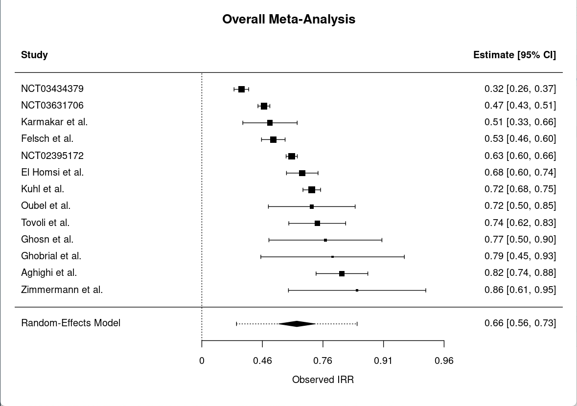
The overall meta-analysis of IRR for RECIST 1.1 yields a pooled \(\kappa\) estimate of 0.66 (95% CI: 0.56 to 0.73), indicating substantial agreement among raters across studies as seen in Figure 3.1. This forest plot illustrates the individual \(\kappa\) estimates for each study, along with their confidence intervals, and the overall pooled estimate. The pooled estimate and associated 95% confidence interval, represented by the black diamond at the bottom, suggests that, on average, raters are able to agree on tumor measurements and classifications with a substantial level of reliability.
However, the analysis also reveals considerable heterogeneity, with a Q statistic of 250.82 (df = 12, p < 0.0001), an I² value of 95.96%, and a tau² of 0.23. These values suggest that nearly all of the observed variability in \(\kappa\) estimates is attributable to real differences between studies rather than chance alone. Such high heterogeneity is not uncommon in meta-analyses of rater agreement, especially when studies differ in design, populations, or rater experience, and it underscores the importance of interpreting the pooled estimate with caution.
For completeness, separate meta-analyses are also conducted for studies reporting Fleiss’ \(\kappa\) and Cohen’s \(\kappa\) individually. The pooled Fleiss’ \(\kappa\) is 0.65 (95% CI: 0.54 to 0.74; Q = 224.23, df = 8, p < 0.0001; I² = 96.80%; tau² = 0.23), and the pooled Cohen’s \(\kappa\) is 0.67 (95% CI: 0.46 to 0.81; Q = 25.22, df = 3, p < 0.0001; I² = 88.48%; tau² = 0.34). These supplemental analyses, along with their corresponding figures, are provided in the appendix. The results for both measures are consistent with the overall finding of substantial inter-rater agreement, though the high heterogeneity persists within each subgroup and is consistent with several of the footnotes in Table 3.1. Meta-analysis plots and funnel plots for Cohen’s \(\kappa\) and Fleiss’ \(\kappa\) are available in the appendix at Figure A.2 and Figure A.1, respectively.
To assess the potential for publication bias, funnel plots are generated for each inter-rater reliability measure included in the meta-analysis as seen in Figure 3.2. This funnel plot displays the individual study estimates of IRR on the x-axis against their standard errors on the y-axis. The studies are represented by points, with the overall pooled estimate indicated by a vertical line. The funnel plot is expected to be symmetric around the pooled estimate if there is no publication bias or small-study effects.
Visual inspection of these plots suggests the presence of asymmetry, raising concerns about apparent publication bias. To formally test for this, Egger’s test for funnel plot asymmetry is performed using the regtest() function from the metafor package. The results of Egger’s test are statistically significant (p = 0.002), providing further evidence that publication bias or small-study effects may be present in the included studies. These findings should be considered when interpreting the pooled estimates, as they indicate that the observed effect sizes may be influenced by factors such as selective reporting or differences in study size.
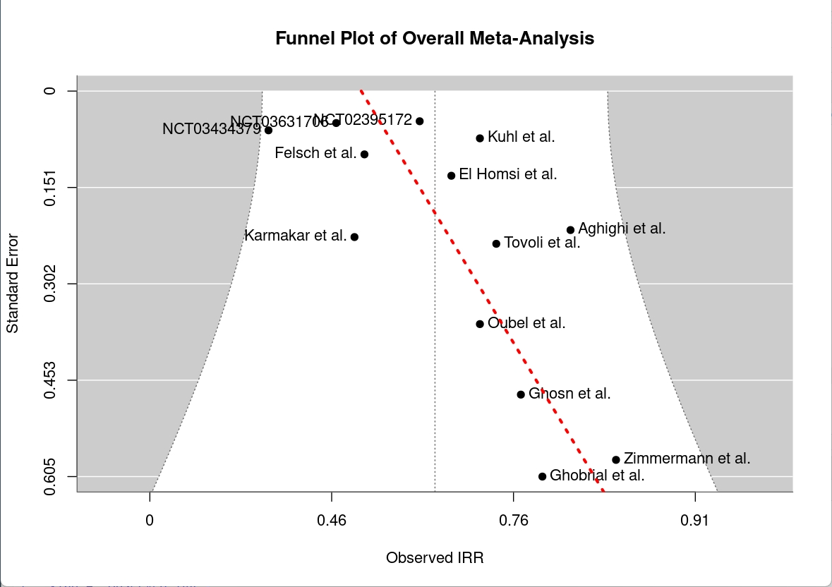
However, the asymmetry observed in the funnel plot should not be interpreted solely as evidence of publication bias. It is likely influenced by the small sample size of the clinical trial data and the fact that all clinical trials were conducted by the same research group. Additionally, Egger’s test is generally recommended for meta-analyses with at least 10 studies, and our analysis includes just slightly over that minimum recommendation at 13. This data limitation should be considered when interpreting the results. Another possible explanation for the observed asymmetry is that the clinical trials may simply have different inter-rater reliability compared to the non-clinical trial studies, potentially reflecting a different underlying “population” of raters than the radiologists used in almost all other studies. This clustering of clinical trials in the funnel plot suggests a potential limitation of the meta-analysis, but does not necessarily indicate publication bias.
More likely, the results reflect small study effects, a common phenomenon in meta-analyses where smaller studies tend to report larger effect sizes than larger studies. Methodological differences may also contribute, as seen in Oubel et al. (8), where raters selected tumors at baseline by consensus rather than independently. This approach can overestimate inter-rater reliability, as consensus selection increases the likelihood of agreement among raters.
An additional observation from the meta-analysis is that the four clinical trials included in the dataset appear to cluster together in terms of effect size, with the funnel plot suggesting these studies are distributed around a different mean (visually estimated at ~0.45) compared to the mean calculated for all studies pooled together. This pattern may indicate that inter-rater reliability is somewhat lower in clinical trial settings than in non-clinical trial contexts. However, this trend is not formally tested for statistical significance due to the small sample size of the clinical trial subgroup. As such, this observation should be interpreted cautiously and considered a potential area for further investigation.
Despite high heterogeneity in the studies and potential small sample bias, the overall findings of the meta-analysis suggest that inter-rater reliability for RECIST 1.1 is moderate to substantial, with a pooled \(\kappa\) estimate of 0.66. Even in the context of clinical trials, where the pooled \(\kappa\) was slightly lower at approximately 0.45, there still appears to be a reasonable level of agreement among raters from a statistical perspective. However, this level of agreement may not be sufficient to ensure consistent and reliable tumor measurements across different raters within a clinical care or trial context, where precise measurements are crucial for treatment decisions and trial outcomes.
The results of our follow-up analyses, particularly the evaluation of differences in hazard ratios and important time-to-event outcomes, thus investigate the practical implications of these findings in clinical trial settings.
3.2 Concordance in Clinical Trial Outcomes
3.2.1 Site Investigators and Central Reviewers Agreement Appears Study-Dependent
To assess inter-rater reliability (IRR), we examine pairwise Cohen’s \(\kappa\) estimates across the studies, as summarized in Table 3.2. This table provides a detailed overview of the pairwise Cohen’s \(\kappa\) estimates, with each column representing a study and each row representing a pairwise comparison between raters. The estimates are presented alongside their 95% confidence intervals and the number of images jointly assessed, providing a clear picture of the level of agreement between the raters in each study. The table also includes the number of cases assessed by each rater, which is important for interpreting the reliability estimates.
In two of the three studies (NCT03434379 and NCT03631706), the highest agreement is observed between the two site investigators, whereas in NCT02395172, this pair has the lowest agreement suggesting potentially high variability or inconsistency in which raters disagree with one another. Moreover, the range of Cohen’s \(\kappa\) values across all studies is broad, from 0.286 to 0.803, further indicating substantial variability in IRR. This variability is consistent with the high heterogeneity observed in the meta-analysis, suggesting that agreement between raters can differ considerably depending on the study context and rater pairings. The pairwise Cohen’s \(\kappa\) estimates provide a useful summary of the level of agreement between raters, but the follow-up analyses using linear mixed effects (LME) models with estimated marginal means (emmeans) provide a more nuanced understanding of the differences between raters.
It is worth explicitly noting that the value in adding these estimated differences on top of the pairwise Cohen’s \(\kappa\) estimates is that they allow us to at least partially account for the quasi-ordinal nature of the RECIST scale. That is, Cohen’s \(\kappa\) penalizes all differences in ratings equally, regardless of whether the differences are of meaning. For example, depending on the context, one might consider stable disease, partial response, and complete response all as sufficient outcomes, but the IRR analysis will necessarily penalize any differences in outcomes by rater. By contrast, using a linear mixed effects model with the RECIST outcomes set to an ordinal scale allowed us to assign a crude numeric value to outcomes that reflect the ordered nature of the scale. This additional layer of analysis can help to clarify the nature of the differences between raters and provide insights into how these differences may impact clinical decision-making or trial outcomes.
| Comparison | NCT02395172 | NCT03434379 | NCT03631706 |
|---|---|---|---|
| Central Reviewer 1 vs Central Reviewer 2 | \(\kappa\) = 0.485 [0.437, 0.534], n=946 | \(\kappa\) = 0.352 [0.284, 0.419], n=466 | \(\kappa\) = 0.513 [0.465, 0.56], n=822 |
| Site Investigator vs Central Reviewer 2 | \(\kappa\) = 0.677 [0.636, 0.719], n=967 | \(\kappa\) = 0.307 [0.233, 0.382], n=425 | \(\kappa\) = 0.424 [0.374, 0.474], n=788 |
| Site Investigator vs Central Reviewer 1 | \(\kappa\) = 0.803 [0.769, 0.836], n=962 | \(\kappa\) = 0.286 [0.211, 0.361], n=424 | \(\kappa\) = 0.49 [0.441, 0.539], n=787 |
Note: While all raters were intended to evaluate the same number of cases, in practice the central reviewers assessed a more complete set of cases than the site investigators. As a result, the central reviewers have more cases represented in the figure.
Full model results for the LMEs are provided in the appendix (Equation A.1, Equation A.2, and Equation A.3), as these are not the primary focus of this section and the point estimates of these models should not be interpreted directly because the RECIST scale can only be considered quasi-ordinal. The main emphasis here, instead, is on the pairwise comparisons of raters using estimated marginal means. As discussed in the Methods (Section 2.2.2.1), the absolute values of these estimates should not be over-interpreted due to the quasi-ordinal nature of the scale; rather, the focus should be on whether the differences are large enough to suggest meaningful disagreement or concordance between raters.
We present here the results of the pairwise comparisons from one of the studies, NCT03631706, in Table 3.3 to demonstrate patterns of disagreement that can occur. The complete set of results for all three studies can be find at Table A.1. This table summarizes the pairwise contrasts of raters from the linear mixed effects model, including the estimated differences in RECIST outcomes, standard errors, degrees of freedom, t-ratios, and p-values. The p-values can be understood as whether a given pairwise comparison is statistically significant, with the Bonferroni method applied to adjust for multiple comparisons. The stars in the p-value column indicate significance levels at \(^{*}p<0.05\), \(^{**}p<0.01\), and \(^{***}p<0.001\).
In the example of NCT03631706, there is a significant difference between the central reviewers as well as a significant difference between the site investigator and central reviewer 1, but no difference between the site investigator and central reviewer 2. Meanwhile, studies NCT02395172 and NCT03434379 show no statistically significant differences between any of the raters, suggesting that the raters are in agreement on the RECIST outcomes for these studies.
| Contrast | Estimate | SE | df | t.ratio | p.value |
|---|---|---|---|---|---|
| Site Inv. - Reader 1 | 0.228 | 0.041 | 2507.766 | 5.630 | 0\(^{***}\) |
| Site Inv. - Reader 2 | 0.064 | 0.041 | 2507.790 | 1.586 | 0.2519\(^{ }\) |
| Reader 1 - Reader 2 | -0.164 | 0.042 | 2501.910 | -3.865 | 3e-04\(^{***}\) |
These results might seem counterintuitive when comparing them to the IRR analyses as, for example, the Cohen’s \(\kappa\) estimates seen in study NCT03434379 might lead one to believe there are substantial differences between the raters. However, the LME analyses suggest that these differences are not statistically significant when accounting for the quasi-ordinal nature of the data, indicating that the raters are generally in agreement on the RECIST outcomes for this study. This discrepancy highlights the importance of considering both pairwise comparisons and more complex modeling approaches when evaluating inter-rater reliability in clinical trials. By employing a combination of methods, we can gain a more comprehensive understanding of how raters interpret and apply the RECIST criteria, ultimately informing efforts to improve consistency and accuracy in tumor response assessment.
3.2.2 Differences Between Raters Extend to Objective Response Rate
While overall agreement between raters is generally acceptable when measuring basic IRR and no differences between raters are identified in two of the three studies when using a mixed modeling strategy, there are notable exceptions in agreement when it comes to evaluating ORR. The omnibus Cochran’s Q test for each study are available in Table 3.4; this table summarizes the results of Cochran’s Q test for ORR analyses across the three studies. The table includes the study name, Cochran’s Q statistic, p-value, and degrees of freedom (df) for each study. The p-values are presented in a format that indicates statistical significance, with stars denoting levels of significance at \(^{*}p<0.05\), \(^{**}p<0.01\), and \(^{***}p<0.001\).
The results of the Cochran’s Q test indicate that there are statistically significant differences in ORR among the raters for studies NCT03434379 and NCT03631706, with p-values less than 0.05 in both cases. This suggests that at least one rater in each of these studies classifies responses differently from the others. To further explore these differences, pairwise McNemar’s post-hoc tests are conducted using the mcnemar.test() function in R, which is appropriate for paired nominal data.
| Study | Cochran’s Q | p-value | df |
|---|---|---|---|
| NCT02395172 | 0.05 | 0.973\(^{ }\) | 2 |
| NCT03434379 | 6.33 | 0.042\(^{*}\) | 2 |
| NCT03631706 | 12.07 | 0.002\(^{**}\) | 2 |
The post-hoc results of the pairwise McNemar’s tests, which provides a chi-squared statistic on 1 degree of freedom, were summarized as p-values in Table 3.5. This table presents the results of the pairwise McNemar comparisons between raters for each study, summarized simply as the p-values of the pairwise comparisons. The p-values are presented in a format that indicates statistical significance after Bonferroni adjustment, with stars denoting levels of significance at \(^{*}p<0.05\), \(^{**}p<0.01\), and \(^{***}p<0.001\). The results indicate that, in NCT03434379, the site investigator disagreed significantly with central reviewer 2 (as indicated by a significant p-value), while in NCT03631706, significant disagreement was observed between the site investigators and both central reviewers. The direction and magnitude of differences between raters can vary across studies, however.
| Study | Central Reviewer 1 vs. Central Reviewer 2 | Site Investigator vs. Central Reviewer 1 | Site Investigator vs. Central Reviewer 2 |
|---|---|---|---|
| NCT02395172 | 1\(^{ }\) | 1\(^{ }\) | 1\(^{ }\) |
| NCT03434379 | 1\(^{ }\) | 0.634\(^{ }\) | 0.048\(^{*}\) |
| NCT03631706 | 1\(^{ }\) | 0.018\(^{*}\) | 0.018\(^{*}\) |
To illustrate how these differences appear in the data itself, contingency table examples for significant and non-significant pairwise comparisons are provided in Table 3.6 and Table 3.7, respectively. That is, the contingency table in Table 3.6 shows how ORR data looks in the event of significant disagreement between raters, namely that the difference between off-diagonal cells is pronounced. On the contrary, the contingency table in Table 3.7 illustrates a lack of significant disagreement, with balanced off-diagonal cell values. (The full set of contingency tables for all studies can be found in the appendix at Table A.2, Table A.3, and Table A.4).
| Site: Response | Site: No Response | |
|---|---|---|
| Central : Response | 55 | 16 |
| Central: No Response | 3 | 72 |
| Site: Response | Site: No Response | |
|---|---|---|
| Central: Response | 268 | 5 |
| Central: No Response | 5 | 50 |
Of particular note in these contingency tables is that the overall number of disagreements between site investigator and central reviewers is relatively low, with most cases showing agreement on whether a response is present or not. This suggests that while there are some differences in how responses are classified, the raters overall accuracy is generally quite high. Based on the contingency table in Table 3.6, one might be tempted to conclude that site investigators are more hesitant to classify someone as having a partial or complete treatment response as an error in this direction could lead to a patient not receiving a treatment that could be beneficial. However, this interpretation should be approached with caution, as the differences in ORR are not necessarily indicative of a systematic bias in one direction or another. In fact, the contingency tables in study NCT03434379 (see Table A.3) show the opposite pattern, with the central reviewers being more likely to classify patients as having a response than the site investigators.
Overall, the results of this sub-analysis further suggest that, when disagreements do occur, they are typically between the site investigator and central reviewers, with the two central reviewers generally in agreement with one another. However, the presence of significant differences between raters in detection of ORR is study-dependent, and the direction of any differences can vary across studies. Moreover, the overall number of disagreements is relatively low, suggesting that while there may be some variability in how responses are classified, the raters overall accuracy is generally quite high. This finding underscores the importance of considering the context and specific characteristics of each study when interpreting inter-rater reliability and agreement on treatment response.
3.2.3 Other Key Trial Outcomes Show No Differences Between Raters
While the ORR analyses reveal some significant differences between raters, it is worth noting that ORR is typically only employed as a secondary outcome and is a more rudimentary measure of treatment response than the more complex time-to-event outcomes. The latter are often more clinically relevant and can provide a more nuanced understanding of treatment effects. In this section, we present the results of time-to-event analyses, which are conducted for three key outcomes: TTP, TTR, and DoR. These analyses are performed using both Kaplan-Meier survival curves and comparison of the hazard ratios derived from Cox proportional hazards models, with the aim of assessing whether there are any significant differences between site investigators and central reviewers in terms of these important clinical endpoints.
Kaplan-Meier curves provide a visual representation of the time-to-event data and are particularly valuable for comparing event rates between different groups—in this case, between assessments made by site investigators versus central reviewers. In these curves, the y-axis represents the probability of being event-free (i.e., survival probability), while the x-axis represents time. For TTP analyses, the event of interest is disease progression, and the curves show the probability of remaining progression-free over time. Similarly, for TTR, the curves display the probability of remaining response-free (i.e., not yet having achieved a response), and for DoR, they show the probability of maintaining a response without progression. When interpreting these curves visually, curves that are higher indicate better outcomes for TTP and DoR (longer time to progression or longer duration of response), while for TTR, a lower curve is preferable (faster time to response). If the curves for different raters overlap substantially, this suggests strong agreement in their assessments. Conversely, separation between curves indicates systematic differences in how raters are evaluating events, with the degree of separation reflecting the magnitude of disagreement. Statistical significance of these visual differences can be assessed using log-rank tests, which evaluate whether the observed separation between curves could have occurred by chance.
Kaplan-Meier survival curves for TTP, TTR, and DoR in study NCT03434379 are shown in Figure 3.3, Figure 3.4, and Figure 3.5, respectively as examples of the time-to-event analyses. Complete results for the three studies including all Kaplain-Meier curves, log(-log(Survival)) plots, and Schoenfeld residuals plots are provided in the appendix at Section A.2.3.1, Section A.2.3.2, and Section A.2.3.3.
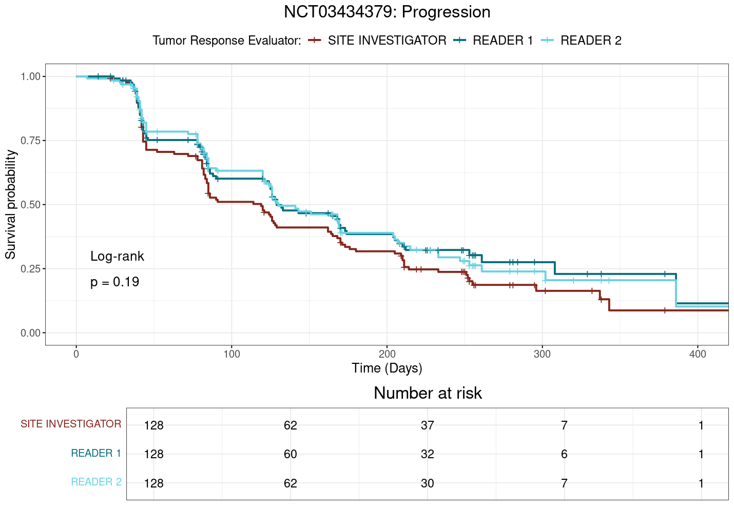
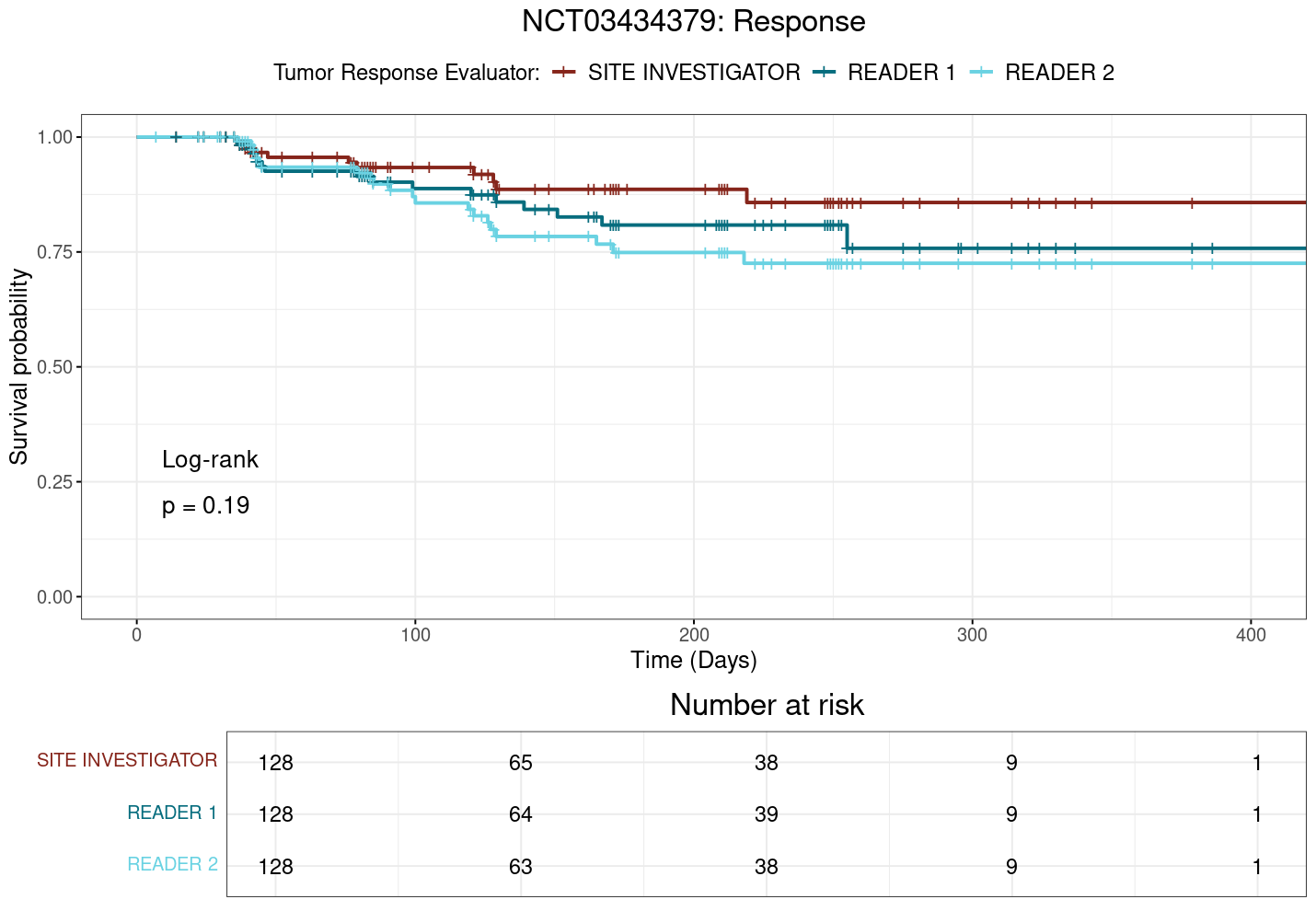
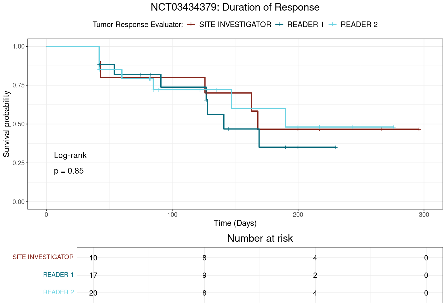
Notably, in study NCT03434379, where significant differences in ORR have been observed in the preceding analyses, the plot TTP (Figure 3.3) suggests that the site investigator may be quicker to assess progression than the central reviewer, as the site investigator’s curve appears to be consistently below that of the central reviewers. Likewise, the site investigator might be slower to identify and classify response to treatment compared to the central reviewer, as indicated by the site investigator’s curve being consistently above that of the central reviewers in the TTR plot (Figure 3.4). However, none of the other studies show such clear differences in time-to-event outcomes between raters, and the overall results suggest that, while there may be some variability in how raters assess time-to-event outcomes, these differences do not appear to be systematic or clinically meaningful.
To more accurately quantify differences in time-to-event outcomes, we employ Cox proportional hazards models to estimate hazard ratios (HRs) for each outcome. We verify the proportional hazards assumption through visual inspection of log(-log(Survival)) plots, which show approximately parallel curves between groups, and Schoenfeld residual plots, which confirm no systematic trends or deviations over time across all outcomes. These diagnostic checks support the validity of our Cox models for subsequent hazard ratio analyses. (The complete set of diagnostic plots for the Cox models, including log(-log(Survival)) plots and Schoenfeld residuals plots, are provided in the appendix at Section A.2.3.)
To formally assess differences in time-to-event outcomes, we calculate the differences in hazard ratios between site investigators and central reviewers for all studies and outcomes. As an aside on interpretation of the values: all differences are calculated as \(\text{Site Investigator} - \text{Central Reviewer}\)1, meaning that a positive difference indicates that the site investigator has a greater hazard ratio and thus a shorter time to event occurrence, while a negative difference indicates that the central reviewer has a greater hazard ratio and thus a shorter time to event occurrence. We avoid interpreting the differences in subjective terms of e.g. “good” or “bad” because the interpretation of these differences is context-dependent and can vary based on the specific clinical scenario, and instead focus on both statistical significance and whether the differences indicate a faster or slower time to event occurrence.
Across all comparisons, no significant differences are found except for a single pairing in study NCT03434379, where the site investigator has a significantly lower hazard ratio for TTR compared to central reviewer 1. This marked difference between raters can be noted in Figure 3.4, which shows the KM survival curves for TTR in NCT03434379. In this case, the site investigator’s curve is consistently and clearly above that of central reviewer 2, indicating a longer time to response for the site investigator (\(p=0.035\)). This is in contrast to the log-rank test results, which do not detect the presence of a statistically significant difference between any groups.
And again, visual inspection of the TTP plot in Figure 3.3 for NCT03434379 suggests that the site investigator may be quicker to assess progression than the central reviewers, as the site investigator’s curve appears to be consistently below that of the central reviewers. This difference is quantified in the calculation of hazard ratios, wherein the site investigator has a greater hazard ratio than the central reviewers. This difference trends towards significance when comparing the site investigator with central reviewer 1 (\(p=0.096\)), but as can be seen in Table 3.8, none of the differences in hazard ratios are statistically significant across the studies for TTP.
| study | Contrast | estimate | SE | p.value |
|---|---|---|---|---|
| NCT02395172 | Site Inv. - Reader 1 | 0.109 | 0.060 | 0.166\(^{ }\) |
| NCT02395172 | Site Inv. - Reader 2 | -0.065 | 0.047 | 0.354\(^{ }\) |
| NCT03434379 | Site Inv. - Reader 1 | 0.242 | 0.117 | 0.096\(^{.}\) |
| NCT03434379 | Site Inv. - Reader 2 | 0.223 | 0.111 | 0.112\(^{ }\) |
| NCT03631706 | Site Inv. - Reader 1 | -0.117 | 0.109 | 0.532\(^{ }\) |
| NCT03631706 | Site Inv. - Reader 2 | 0.069 | 0.100 | 0.773\(^{ }\) |
| study | Contrast | estimate | SE | p.value |
|---|---|---|---|---|
| NCT02395172 | Site Inv. - Reader 1 | 0.000 | 0.106 | 1\(^{ }\) |
| NCT02395172 | Site Inv. - Reader 2 | 0.006 | 0.060 | 0.995\(^{ }\) |
| NCT03434379 | Site Inv. - Reader 1 | -0.441 | 0.317 | 0.346\(^{ }\) |
| NCT03434379 | Site Inv. - Reader 2 | -0.667 | 0.269 | 0.035\(^{*}\) |
| NCT03631706 | Site Inv. - Reader 1 | 0.112 | 0.092 | 0.44\(^{ }\) |
| NCT03631706 | Site Inv. - Reader 2 | 0.069 | 0.089 | 0.719\(^{ }\) |
| study | Contrast | estimate | SE | p.value |
|---|---|---|---|---|
| NCT02395172 | Site Inv. - Reader 1 | -0.068 | 0.187 | 0.931\(^{ }\) |
| NCT02395172 | Site Inv. - Reader 2 | 0.151 | 0.176 | 0.666\(^{ }\) |
| NCT03434379 | Site Inv. - Reader 1 | -0.275 | 0.520 | 0.858\(^{ }\) |
| NCT03434379 | Site Inv. - Reader 2 | -0.036 | 0.523 | 0.997\(^{ }\) |
| NCT03631706 | Site Inv. - Reader 1 | -0.068 | 0.237 | 0.955\(^{ }\) |
| NCT03631706 | Site Inv. - Reader 2 | 0.332 | 0.263 | 0.417\(^{ }\) |
More generally, only one statistically significant difference in hazard ratios is found across all studies and outcomes, which is for TTR in NCT03434379. This suggests that, while there may be some variability in how raters assess time-to-event outcomes, these differences do not generally appear to be statistically or clinically relevant for an individual study. The results of the hazard ratio analyses are summarized in Table 3.8, Table 3.9, and Table 3.10 for TTP, TTR, and DoR, respectively.
Although few if any individual differences are found between the site investigators and central reviewers in terms of time to event outcomes, it remains possible that small, systematic differences could be detected with a larger sample size of studies and raters. To address this, meta-analyses of the time-to-event outcomes are conducted, explored in the next section. These meta-analyses aim to determine whether any systematic differences between site investigators and central reviewers could be identified across multiple studies, thereby providing a more robust assessment of inter-rater reliability for RECIST 1.1 in clinical trial settings.
3.2.4 Meta-Analyses Confirm Lack of Differences Between Raters
The meta-analyses of time-to-event outcomes (TTP, TTR, and DoR) reveal no statistically significant differences between site investigators and central reviewers across studies. The forest plots in Figure 3.6, Figure 3.7, and Figure 3.8 illustrate the pooled hazard ratios for each outcome, with the central vertical line indicating no difference (\(\Delta HR=0\)). The squares represent the point estimates of the hazard ratios for each study, with the size of the square proportional to the weight of the study in the meta-analysis. The horizontal lines extending from each square represent the 95% confidence intervals for the hazard ratios, and the diamond at the bottom represents the pooled estimate across all studies. A diamond that does not cross the vertical line indicates a statistically significant difference, while a diamond that crosses the line indicates no significant difference.
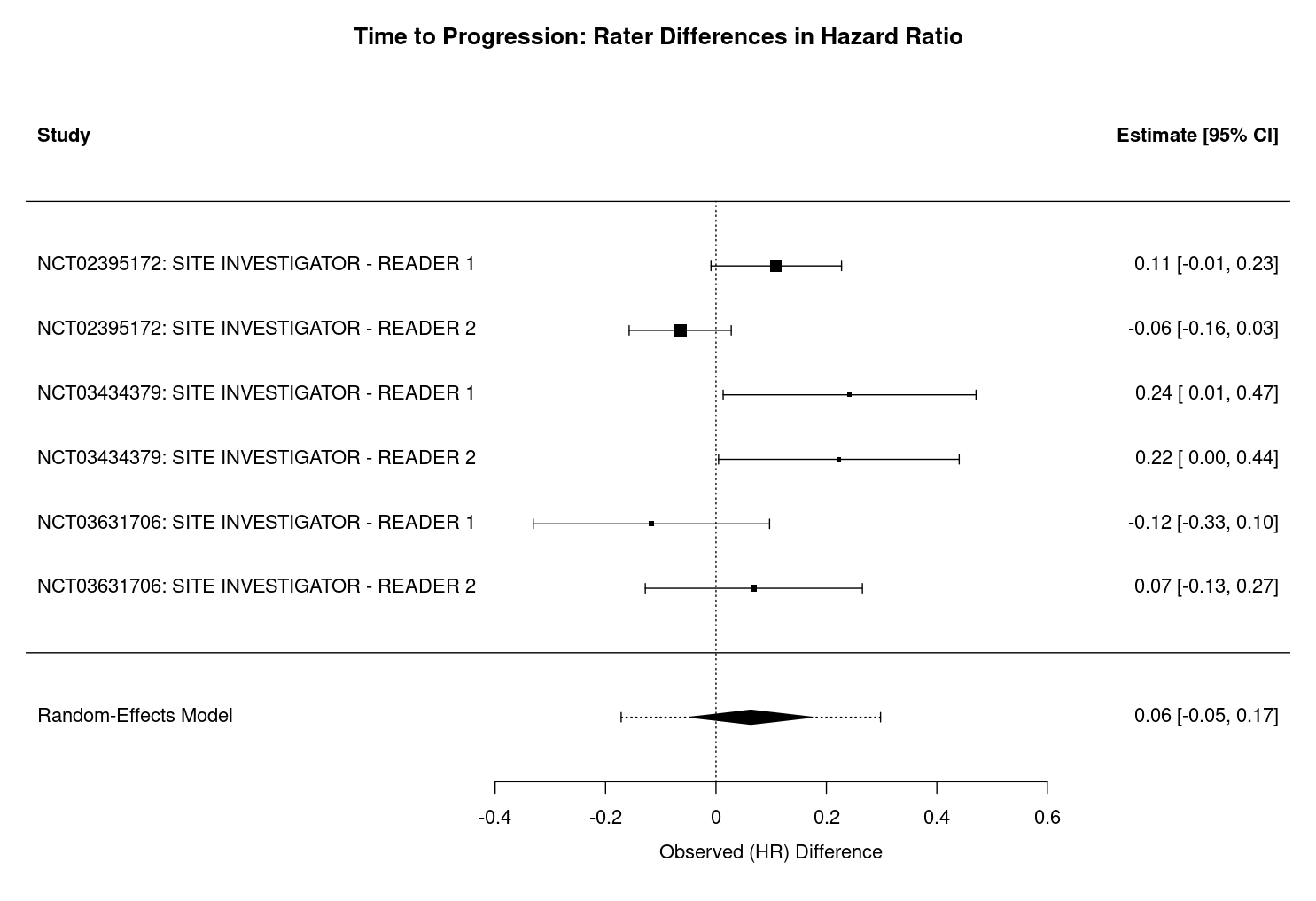
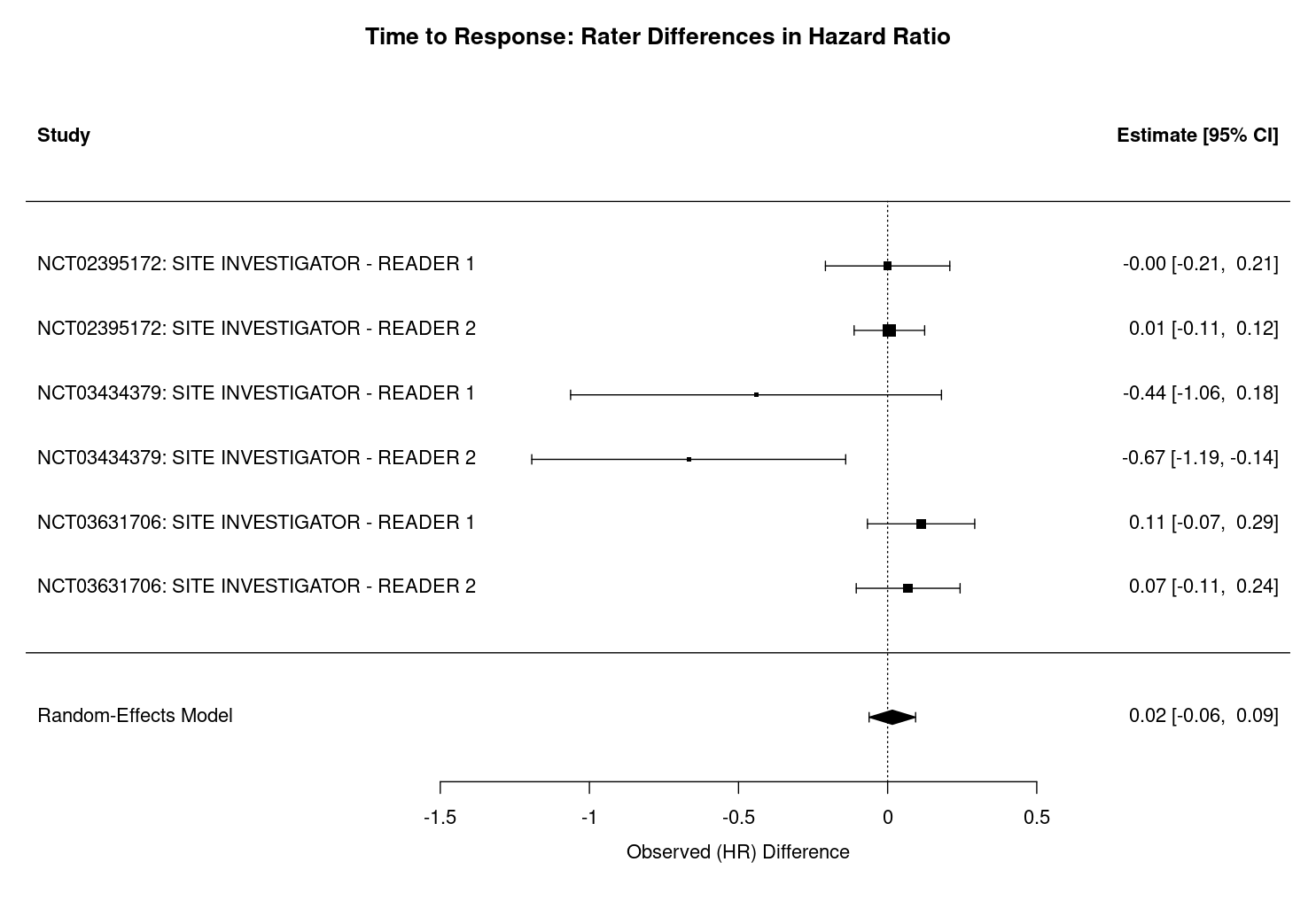
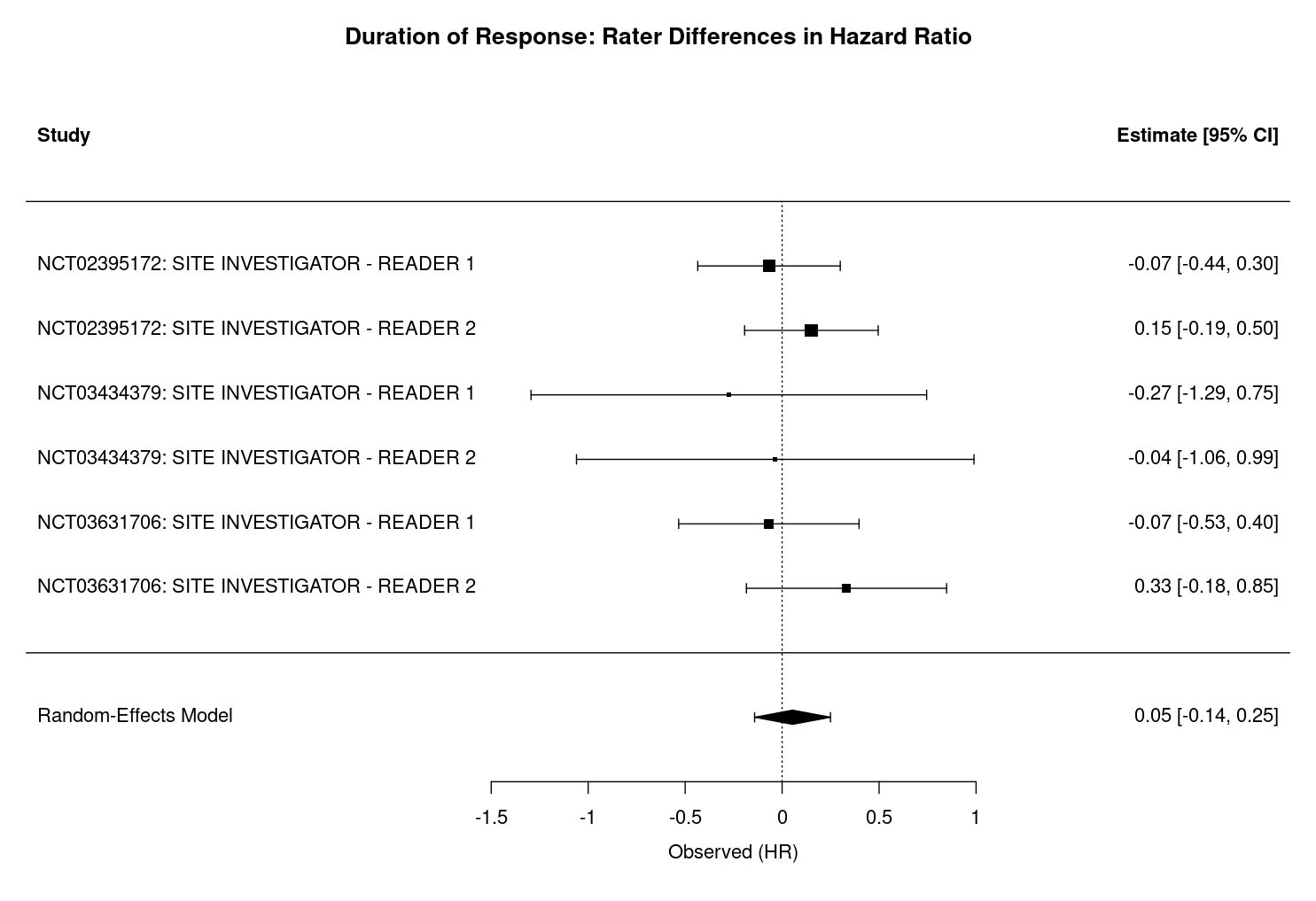
For each outcome, the pooled difference in hazard ratios is small and the 95% confidence intervals include zero, indicating a lack of systematic bias between rater groups. Specifically, for TTP, the difference in hazard ratios is 0.06 (95% CI: -0.05 to 0.17, p = 0.262, Figure 3.6), with moderate heterogeneity (I² = 63.4%, τ² = 0.0112, heterogeneity p = 0.0155, df = 5). For TTR, the difference is 0.02 (95% CI: -0.06 to 0.09, p = 0.691, Figure 3.7), with negligible heterogeneity (I² = 0.01%, τ² = 0.0000, heterogeneity p = 0.0739, df = 5). For DoR, the difference is 0.05 (95% CI: -0.14 to 0.25, p = 0.590, Figure 3.8), with no observed heterogeneity (I² = 0.0%, τ² = 0.0000, heterogeneity p = 0.771, df = 5).
Interpretation of the heterogeneity statistics further supports these findings. The I² statistic quantifies the percentage of total variation across studies attributable to heterogeneity rather than chance. For TTP, an I² of 63.4% indicates moderate heterogeneity, suggesting that some observed differences in hazard ratios may reflect real differences between studies. In contrast, I² values near zero for TTR and DoR indicate that almost all variability is due to sampling error rather than true heterogeneity. The τ² statistic represents the estimated between-study variance in true effect sizes, with higher values (as in TTP) indicating more variability in underlying effects, and values near zero (as in TTR and DoR) indicating little to no between-study variance. The heterogeneity test p-value, derived from Cochran’s Q test, assesses whether observed variability in effect sizes exceeds what would be expected by chance. A significant p-value (e.g., p = 0.0155 for TTP) suggests real heterogeneity, while non-significant values (as in TTR and DoR) indicate no evidence of excess heterogeneity.
Across all outcomes, positive values indicate that site investigators tend to report slightly higher hazard ratios than central reviewers, suggesting more rapid assessments of progression, response, or shorter durations of response. However, as previously noted, none of these differences reach statistical significance i.e. the 95% confidence intervals for all outcomes include zero.
Although none of the meta-analyses reach significance, it is still worthwhile noting that not all data points are fully independent, as each study contributes two sets of central reviewer–site investigator pairs. This could potentially double-weight some trials and narrow confidence intervals. Nevertheless, the consistent lack of significant differences across outcomes supports the robustness of these findings. In larger meta-analyses or those with more diverse reviewer groups, the non-independence of central reviewers who likely share training, software, and protocols should be considered when interpreting results.
3.2.5 Equivalence Between Raters Established for TTR and TTP
To formally assess whether the outcomes measured by site investigators and central reviewers could be considered equivalent, we apply the TOST procedure to the differences in hazard ratios for TTP, TTR, and DoR. The equivalence bounds are set a priori as hazard ratios (HRs) of 0.8 to 1.25, which correspond to -0.223 to 0.223 on the log scale. These bounds represent the range of differences that would be considered not clinically meaningful, and thus, if the 90% confidence interval for the difference in log hazard ratios falls entirely within this interval, equivalence can be concluded.
The TOST plots in Figure 3.9, Figure 3.10, and Figure 3.11 summarize the results of the TOST procedure for TTP, TTR, and DoR, respectively. These plots provide a visual framework for interpreting equivalence testing results. In each plot, the dashed vertical lines represent the equivalence bounds of -0.223 to 0.223 on the log scale (corresponding to HRs of 0.8 to 1.25). The area between these lines defines the region of practical equivalence. If the 90% confidence interval for the difference in means (represented by the horizontal line with the point estimate as a dot) lies entirely within this region, equivalence is supported. If the confidence interval crosses either bound, however, equivalence cannot be established.
Our analyses show distinct patterns across the three outcomes. For TTP and TTR, the confidence intervals are fully contained within the equivalence bounds, providing strong evidence of practical equivalence between site investigators and central reviewers for these outcomes. In contrast, the DoR interval marginally exceeds the upper equivalence bound, suggesting that while the difference is likely small, we cannot formally conclude equivalence for this outcome with the available data.
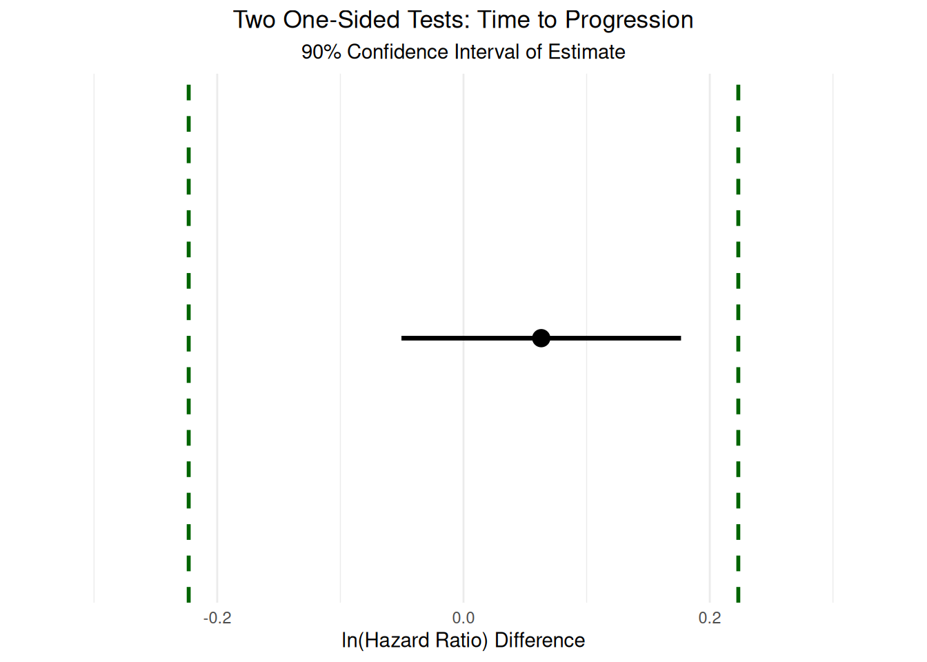
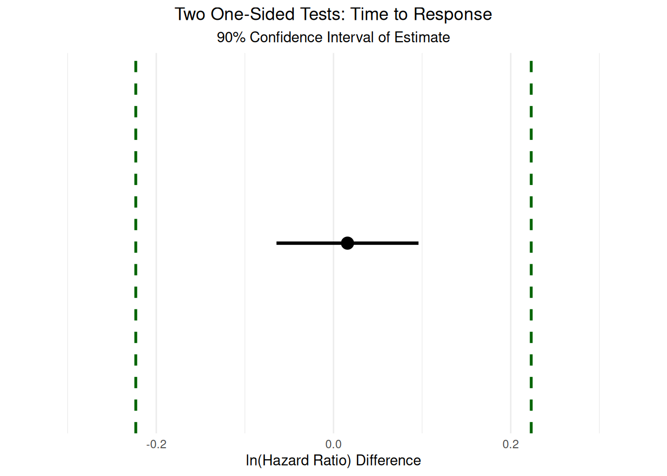
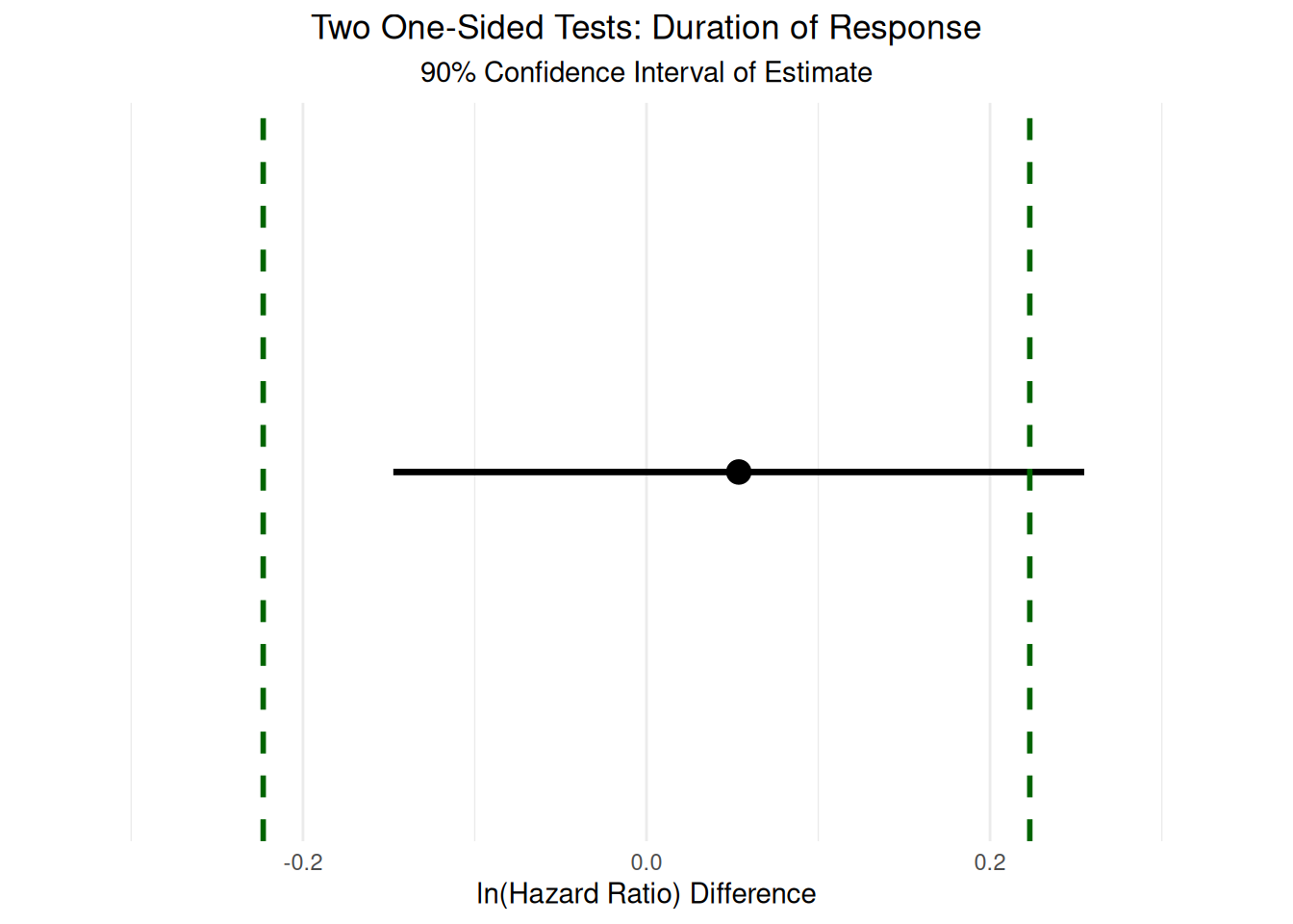
The quantitative TOST analyses indicate that both TTP and TTR are statistically equivalent between site investigators and central reviewers. For TTP, the 90% confidence interval for the difference in log hazard ratios is [-0.05, 0.177], with an equivalence test result of t(5) = -2.840 and a p-value of 0.0181. For TTR, the 90% confidence interval is [-0.064, 0.096], with t(5) = -5.214 and a p-value of 0.00171. In both cases, the confidence intervals fall entirely within the equivalence bounds, supporting the conclusion that any differences between site investigators and central reviewers are not clinically meaningful for these outcomes. In contrast, for DoR, the 90% confidence interval is [-0.147, 0.255] with t(5) = -1.697 and a p-value of 0.0752. Here, the upper bound of the confidence interval slightly exceeds the equivalence margin, and thus formal equivalence cannot be established. However, the interval is close to the bounds, suggesting that the two groups likely have similar durations of response, but the available data do not provide sufficient certainty to draw a definitive conclusion.
It is important to note several limitations when interpreting these results. First, the number of studies and events included in the DoR analysis is limited, resulting in wider confidence intervals and reduced statistical power to detect equivalence. This limitation is common in meta-analyses of clinical trial endpoints, especially for outcomes that are less frequently observed or reported. Second, the choice of equivalence bounds, while based on conventional thresholds for clinical relevance, remains somewhat arbitrary and may not capture all perspectives on what constitutes a meaningful difference. Finally, the TOST procedure assumes that the data are sufficiently powered to detect equivalence; in cases where sample sizes are small, failure to demonstrate equivalence may reflect limited data rather than true differences between groups.
Overall, these results provide strong evidence that site investigators and central reviewers yield equivalent results for TTP and TTR, and likely similar results for DoR, though the latter cannot be confirmed with high confidence. These findings support the robustness of RECIST-based time-to-event endpoints to rater differences in the context of clinical trials, but also highlight the need for larger studies to more definitively assess equivalence for less common outcomes such as DoR.
3.3 RECIST Thresholds are Robust
This section presents a series of sensitivity analyses designed to evaluate how key trial outcomes respond to changes in the RECIST thresholds for disease progression and partial response. For each analysis, we systematically recalculate RECIST-based outcomes using the available SLD data, varying the progression and response thresholds across a plausible range from [0, 100]%. The results are visualized as heatmaps, which provide an intuitive summary of how inter-rater reliability, objective response rate, and time-to-event outcomes shift as the thresholds are altered.
In these heatmaps, the axes represent the progression and partial response thresholds, while the color scale indicates either the deviation from the original estimate (for IRR and time-to-event outcomes) or the p-value from Cochran’s Q test (for ORR). Rather than focusing on statistical significance at each point, these visualizations are intended to highlight the overall sensitivity or robustness of the outcomes to threshold selection. Regions of stability, sensitivity, or missing data can be readily identified, allowing for a nuanced interpretation of how RECIST criteria perform under different assumptions. Full details for interpreting each heatmap are provided in the relevant sub-sections below.
It is also important to note that, in the cases of ORR and TTR, changes in the threshold values for progression do not affect the corresponding heatmaps, and similarly, changes in the threshold values for partial response do not affect the heatmaps for TTP. Despite this, all heatmaps were plotted with both dimensions to provide a consistent visual scale for comparison across outcomes. This approach allows readers to directly compare the sensitivity of different endpoints to threshold selection, even when one axis does not influence a particular outcome.
3.3.1 IRR Shows Stability Across Thresholds
The IRR sensitivity analyses, visualized as heatmaps, illustrate how inter-rater reliability responds to changes in the RECIST thresholds for disease progression and partial response. For both the Target Lesion and Overall Outcome, the heatmaps display values relative to the original IRR calculated at the standard RECIST criteria (20% progression, 30% response), with intersecting black lines marking these reference thresholds. Negative values indicate a decrease in IRR compared to the original, while positive values indicate an increase.
For the Target Lesion outcome, the heatmaps (see Figure 3.12) show a clear trend: as either threshold approaches 100%, \(\kappa\) values decrease. This is expected, as very few cases are classified as having a response or progression at such extreme thresholds, reducing the opportunity for agreement between raters. Additionally, in clinical trials, patients are typically removed from the study once progression is observed, making high progression thresholds less relevant and further limiting available data in these regions. Aside from this expected decline at the extremes, the heatmaps for the Target Lesion outcome do not display systematic patterns across studies, suggesting that IRR is generally stable across a wide range of plausible threshold values.
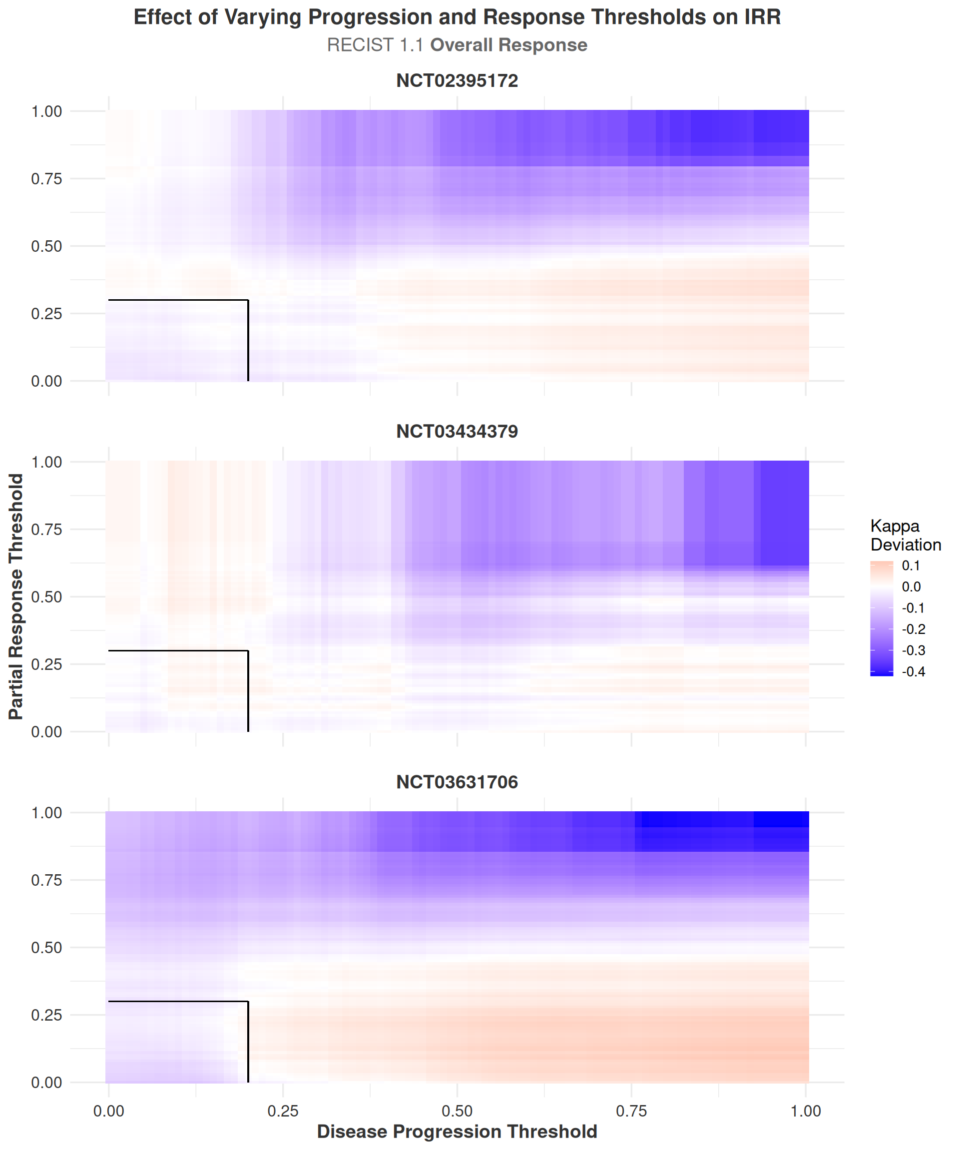
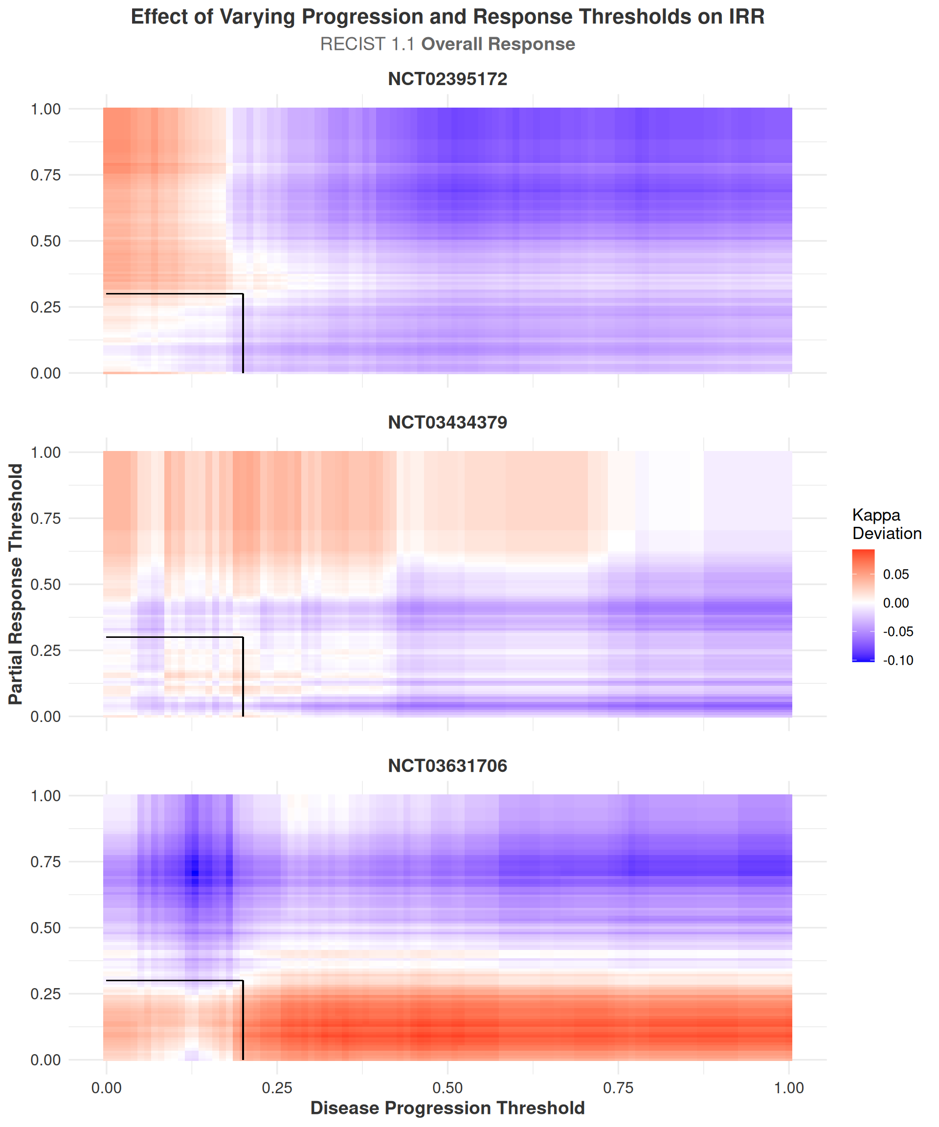
The Overall Outcome is a composite measure that incorporates information from the Target Lesion, Non-Target Lesion, and New Lesion outcomes, providing a more comprehensive assessment of tumor response. The heatmaps for the Overall Outcome (Figure 3.13) display a similar lack of systematic trends or abrupt changes in IRR as thresholds are varied. Notably, the deviation in \(\kappa\) for the heatmaps of target lesions ranges from -0.422 to 0.119, while the deviation in \(\kappa\) for th heatmaps of overall response ranges from -0.103 to 0.093. This indicates that IRR can be somewhat sensitive to changes in the RECIST thresholds used for calculating the Target outcome, particularly at extreme values, but the IRR for Overall response is well-stabilized by the information gain from non-target and new lesions.
The much smaller range of \(\kappa\) deviations in the overall outcome heatmaps suggests that the RECIST criteria are robust to changes in the thresholds for disease progression and response, and that the overall IRR is not significantly affected by these changes. This robustness supports the reliability of RECIST when applied in a comprehensive manner across different studies and raters.
3.3.2 ORR Unaffected by RECIST Thresholds
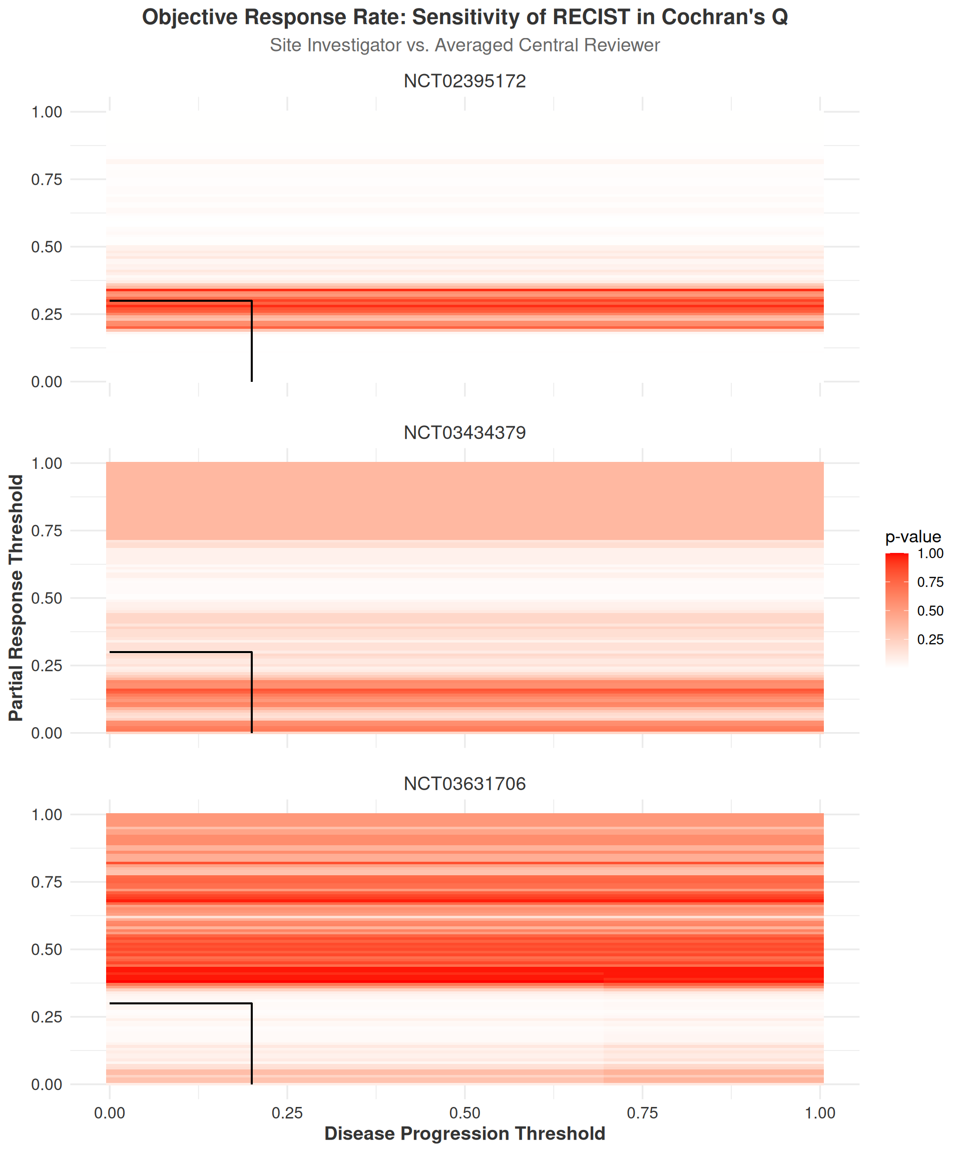
The interpretation of ORR heatmaps differs from the IRR analyses in that we focus on p-values from Cochran’s Q tests rather than differences in effect estimates. This approach is selected because comparing differences in p-values across thresholds has limited interpretive value without constant reference to the conventional alpha threshold of 0.05. Instead, our analysis aims to identify regions where statistically significant differences might emerge either within or across studies as thresholds change.
While more precise statistical analyses could be performed by selecting specific clinically relevant thresholds for progression and partial response, then conducting targeted pairwise comparisons between raters at these points, such an approach would require a priori hypotheses about optimal thresholds. Without such predefined hypotheses, we instead utilized heatmaps as a visualization tool to comprehensively examine the sensitivity of ORR measurements to changes in RECIST thresholds and their subsequent effect on inter-rater differences.
For all outcomes studied in this analysis, seen in Figure 3.14, we observed no systematic changes in Cochran’s Q p-values across the range of RECIST thresholds. For example, in study NCT02395172, the p-values within about \(\pm\) 10% of the original response threshold remained consistently above the conventional alpha threshold of 0.05, indicating no significant differences between raters. However, nearly the opposite pattern was observed in NCT03631706, where p-values were consistently below or near 0.05 within \(\pm\) 10% of the original response threshold. Above all, given the relatively small number of participants who reached a disease response at the original threshold, it is likely reasonable to conclude that most of the variation seen within plots here is due to sampling error rather than systematic differences between raters.
3.3.3 Time-to-Event Outcomes Show no Patterns Across Changing Thresholds
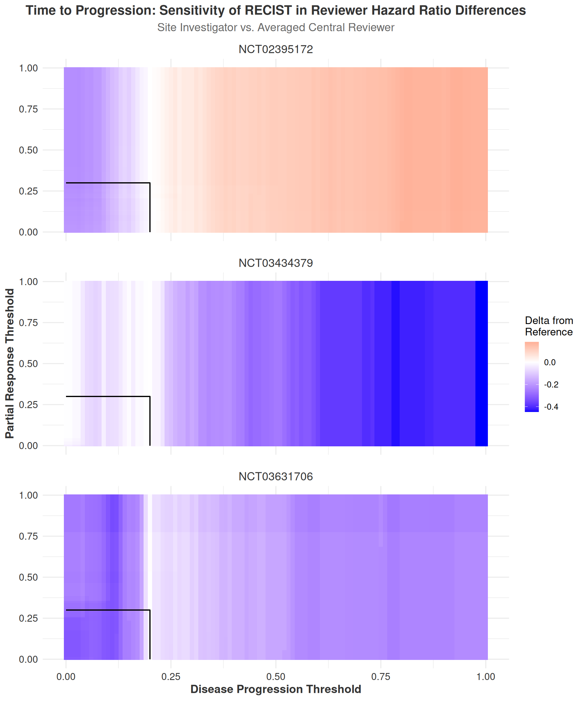
To evaluate how classification threshold changes influenced the estimated risk associated with reviewer assessments across the time-to-event outcomes, we conducted a difference-in-differences (DiD) analysis comparing hazard ratios between site investigators and central reviewers. In all Cox proportional hazards models, the site investigator served as the reference group, and thus their hazard ratio remained constant across thresholds. The central reviewer’s hazard ratio, by contrast, varied depending on changes in the RECIST thresholds for disease progression and response.
As noted in the Methods section in Equation 2.14, the calculations for the DiD analysis can be simplified to the following equation:
\[ \begin{aligned} \Delta_{\text{RECIST}} - \Delta_{\text{Sensitivity}} &= HR_{\text{Central Reviewer New}} - HR_{\text{Central Reviewer Original}} \end{aligned} \]
where \(\Delta_{\text{RECIST}}\) represents the difference in hazard ratios between the site investigator and central reviewer at the original RECIST thresholds, and \(\Delta_{\text{Sensitivity}}\) represents the difference in hazard ratios at any given new threshold. The DiD value thus represents the change in the central reviewer’s hazard ratio relative to the site investigator’s hazard ratio as the RECIST thresholds are varied.
A positive DiD value indicates that the central reviewer’s hazard ratio increased under the new threshold. Conversely, a negative DiD suggests that the central reviewer’s estimated hazard decreased under the new classification rule. Additionally, it should again be noted that we refer here to a single central reviewer because we have averaged the hazard ratios of the two central reviewers within each study. This averaging was done to simplify the analysis and interpretation, as the two central reviewers generally agreed closely in their hazard ratio estimates and the display and interpretation of such results would have been unwieldy.
The TTP heatplot (Figure 3.15) shows generally decreasing values of DiD both when the disease progression threshold is increased and decreased with the exception of study NCT02395172. In this study, the DiD values slightly increased as the progression threshold was raised. The general overall decreases in DiD values indicate that the central reviewers showed, on average, a decrease in their estimated hazard ratios relative to the site investigators as the disease progression threshold was increased (i.e. the discrepancy in HRs between the site investigator and central reviewer hazard ratios decreased). However, changes in any direction are not generally noticeable at all within \(\sim\pm5\%\) of the original progression threshold, and large decreases in DiD values are only observed at the extremes of the progression threshold range. This suggests that the RECIST thresholds for disease progression are robust to changes in the progression threshold, and that the differences between raters would not be expected to change significantly with small changes in the progression threshold.
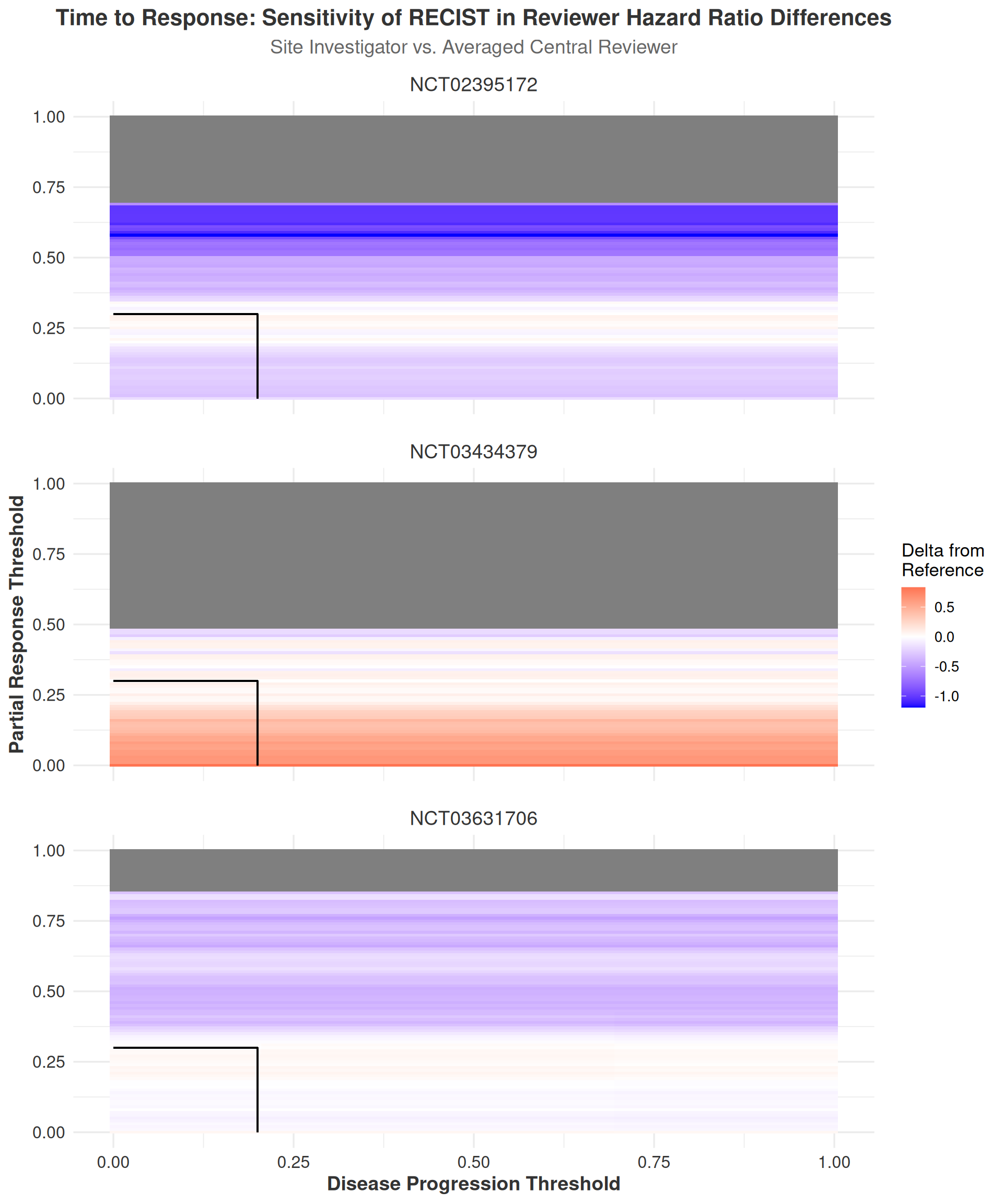
Regarding the TTR and DoR sensitivity analyses, it is important to first note that the TTR and DoR heatmaps contain extensive regions of missing data points. This occurs due to the filtering procedure outlined in the Methods section (Section 2.2.3.1), where data sets with fewer than \((k-1)*10\) cases were excluded, with \(k\) representing the number of raters in the study. This filtering process ensures that a reasonable number of events are present in each data set to allow for meaningful comparisons between raters. While heatmaps without such filtering are available in the appendix (Figure A.33, Figure A.34), they are not included in the main text as they do not provide additional insights beyond what is already presented here. Furthermore, some of the observed DiD values in the unfiltered maps are extremely large (exceeding an HR of 15 in some cases), making them difficult to interpret in a meaningful clinical context.
With these considerations in mind, the results of the TTR sensitivity analyses in (Figure 3.16) generally mirror those of the TTP sensitivity analyses, with the notable exception that the DiD values for TTR tend to be larger in magnitude. This increased range of DiD values likely stems from the fact that TTR events are generally less frequent than TTP events, making the DiD values more sensitive to changes in the RECIST thresholds. This interpretation is supported by the observation that up to 50% of the data points in the TTR heatmaps are missing due to the filtering procedure, while the TTP heatmaps maintain complete data coverage because a sufficient number of progression events were observed at all threshold combinations.
Interpretation of the DoR heatmaps (Figure 3.17) follows a pattern almost identical to that of the TTR heatmaps, with both displaying similar ranges of DiD values and similar patterns across the RECIST thresholds. The DoR heatmaps also exhibit a large number of missing data points due to the filtering procedure, but with an important distinction: missing data points are visible across both dimensions of the heatmap. This occurs because the DoR outcome requires both an identified response event and a subsequent progression event to calculate a duration of response. Consequently, at certain thresholds, response may be observed without progression, leading to an apparent step-down pattern from left to right in the heatmaps. This pattern is particularly pronounced in study NCT03631706.
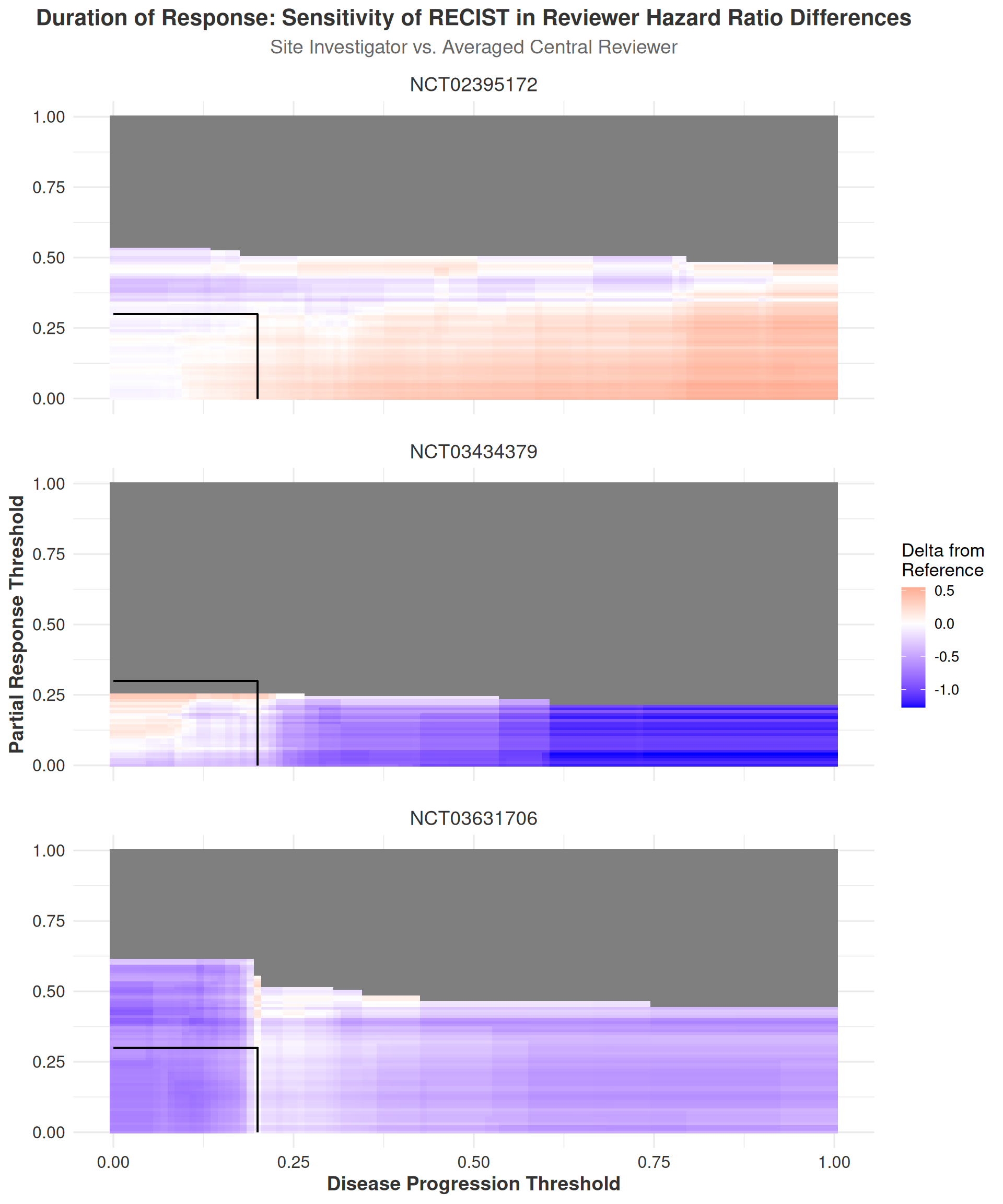
Collectively, the time-to-event sensitivity analyses provide strong evidence that the RECIST thresholds for disease progression and response are robust to changes in the thresholds, with differences between raters remaining largely unaffected by threshold adjustments. These findings align with the results from both the IRR and ORR analyses, which similarly suggest that the RECIST criteria demonstrate general robustness to threshold changes and that differences between raters are neither systematic nor clinically meaningful. The heatmaps offer a clear visual representation of these findings, facilitating identification of regions where the RECIST thresholds exhibit stability or sensitivity to changes in the progression and response parameters.
In general, the DiD analyses reveal minimal systematic differences between site investigators and central reviewers across the range of RECIST thresholds examined, with exceptions occurring only at extreme threshold values. This pattern reinforces the conclusion that the RECIST criteria are robust to threshold adjustments and that differences between raters remain clinically insignificant across a reasonable range of threshold values. Overall, these sensitivity analyses provide compelling evidence for the reliability of RECIST-based time-to-event endpoints in clinical trials, supporting confidence in their continued use for assessing treatment response.
Cox modeling is done with the raters set as a factor (i.e. ordinal) variable in R with Site Investigator as the reference value. Thus, its estimate is always 0, the other raters’ HRs are relative to this value, and the direction of the difference indicates whether the site investigator has a greater or lesser hazard ratio than the central reviewers.↩︎